Schelling's segregation model
In this introductory example we demonstrate Agents.jl's architecture and features through building the following definition of Schelling's segregation model:
- Agents belong to one of two groups (0 or 1).
- The agents live in a two-dimensional Chebyshev grid (8 neighbors per position).
- If an agent is in the same group with at least three neighbors, then it is happy.
- If an agent is unhappy, it keeps moving to new locations until it is happy.
Schelling's model shows that even small preferences of agents to have neighbors belonging to the same group (e.g. preferring that at least 30% of neighbors to be in the same group) could lead to total segregation of neighborhoods.
This model is also available as Models.schelling.
Defining the agent type
using Agents, Plots

mutable struct SchellingAgent <: AbstractAgent
    id::Int # The identifier number of the agent
    pos::Dims{2} # The x, y location of the agent on a 2D grid
    mood::Bool # whether the agent is happy in its position. (true = happy)
    group::Int # The group of the agent,  determines mood as it interacts with neighbors
end
Notice that the position of this Agent type is a Dims{2}, equivalent to NTuple{2,Int}, because we will use a 2-dimensional GridSpace.
We added two more fields for this model, namely a mood field which will store true for a happy agent and false for an unhappy one, and an group field which stores 0 or 1 representing two groups.
Notice also that we could have taken advantage of the macro @agent (and in fact, this is recommended), and defined the same agent as:
@agent SchellingAgent GridAgent{2} begin
    mood::Bool
    group::Int
end
Creating a space
For this example, we will be using a Chebyshev 2D grid, e.g.
space = GridSpace((10, 10), periodic = false)GridSpace with size (10, 10), metric=chebyshev and periodic=false
Creating an ABM
To make our model we follow the instructions of AgentBasedModel. We also want to include a property min_to_be_happy in our model, and so we have:
properties = Dict(:min_to_be_happy => 3)
schelling = ABM(SchellingAgent, space; properties)
AgentBasedModel with 0 agents of type SchellingAgent space: GridSpace with size (10, 10), metric=chebyshev and periodic=false scheduler: fastest properties: Dict(:min_to_be_happy => 3)
Here we used the default scheduler (which is also the fastest one) to create the model. We could instead try to activate the agents according to their property :group, so that all agents of group 1 act first. We would then use the scheduler property_activation like so:
schelling2 = ABM(
    SchellingAgent,
    space;
    properties = properties,
    scheduler = property_activation(:group),
)
AgentBasedModel with 0 agents of type SchellingAgent space: GridSpace with size (10, 10), metric=chebyshev and periodic=false scheduler: by_property properties: Dict(:min_to_be_happy => 3)
Notice that property_activation accepts an argument and returns a function, which is why we didn't just give property_activation to scheduler.
Creating the ABM through a function
Here we put the model instantiation in a function so that it will be easy to recreate the model and change its parameters.
In addition, inside this function, we populate the model with some agents. We also change the scheduler to random_activation. Because the function is defined based on keywords, it will be of further use in paramscan below.
function initialize(; numagents = 320, griddims = (20, 20), min_to_be_happy = 3)
    space = GridSpace(griddims, periodic = false)
    properties = Dict(:min_to_be_happy => min_to_be_happy)
    model = ABM(SchellingAgent, space;
                properties = properties, scheduler = random_activation)
    # populate the model with agents, adding equal amount of the two types of agents
    # at random positions in the model
    for n in 1:numagents
        agent = SchellingAgent(n, (1, 1), false, n < numagents / 2 ? 1 : 2)
        add_agent_single!(agent, model)
    end
    return model
end
Notice that the position that an agent is initialized does not matter in this example. This is because we use add_agent_single!, which places the agent in a random, empty location on the grid, thus updating its position.
Defining a step function
Finally, we define a step function to determine what happens to an agent when activated.
function agent_step!(agent, model)
    agent.mood == true && return # do nothing if already happy
    minhappy = model.min_to_be_happy
    neighbor_positions = nearby_positions(agent, model)
    count_neighbors_same_group = 0
    # For each neighbor, get group and compare to current agent's group
    # and increment count_neighbors_same_group as appropriately.
    for neighbor in nearby_agents(agent, model)
        if agent.group == neighbor.group
            count_neighbors_same_group += 1
        end
    end
    # After counting the neighbors, decide whether or not to move the agent.
    # If count_neighbors_same_group is at least the min_to_be_happy, set the
    # mood to true. Otherwise, move the agent to a random position.
    if count_neighbors_same_group ≥ minhappy
        agent.mood = true
    else
        move_agent_single!(agent, model)
    end
    return
end
For the purpose of this implementation of Schelling's segregation model, we only need an agent step function.
When defining agent_step!, we used some of the built-in functions of Agents.jl, such as nearby_positions that returns the neighboring position on which the agent resides, ids_in_position that returns the IDs of the agents on a given position, and move_agent_single! which moves agents to random empty position on the grid. A full list of built-in functions and their explanations are available in the API page.
Stepping the model
Let's initialize the model with 370 agents on a 20 by 20 grid.
model = initialize()AgentBasedModel with 320 agents of type SchellingAgent space: GridSpace with size (20, 20), metric=chebyshev and periodic=false scheduler: random_activation properties: Dict(:min_to_be_happy => 3)
We can advance the model one step
step!(model, agent_step!)Or for three steps
step!(model, agent_step!, 3)Running the model and collecting data
We can use the run! function with keywords to run the model for multiple steps and collect values of our desired fields from every agent and put these data in a DataFrame object. We define vector of Symbols for the agent fields that we want to collect as data
adata = [:pos, :mood, :group]

model = initialize()
data, _ = run!(model, agent_step!, 5; adata)
data[1:10, :] # print only a few rows| step | id | pos | mood | group | |
|---|---|---|---|---|---|
| Int64 | Int64 | Tuple… | Bool | Int64 | |
| 1 | 0 | 1 | (18, 15) | 0 | 1 |
| 2 | 0 | 2 | (1, 18) | 0 | 1 |
| 3 | 0 | 3 | (11, 2) | 0 | 1 |
| 4 | 0 | 4 | (14, 19) | 0 | 1 |
| 5 | 0 | 5 | (15, 8) | 0 | 1 |
| 6 | 0 | 6 | (13, 18) | 0 | 1 |
| 7 | 0 | 7 | (4, 2) | 0 | 1 |
| 8 | 0 | 8 | (12, 11) | 0 | 1 |
| 9 | 0 | 9 | (6, 8) | 0 | 1 |
| 10 | 0 | 10 | (11, 18) | 0 | 1 |
We could also use functions in adata, for example we can define
x(agent) = agent.pos[1]
model = initialize()
adata = [x, :mood, :group]
data, _ = run!(model, agent_step!, 5; adata)
data[1:10, :]| step | id | x | mood | group | |
|---|---|---|---|---|---|
| Int64 | Int64 | Int64 | Bool | Int64 | |
| 1 | 0 | 1 | 17 | 0 | 1 |
| 2 | 0 | 2 | 12 | 0 | 1 |
| 3 | 0 | 3 | 16 | 0 | 1 |
| 4 | 0 | 4 | 20 | 0 | 1 |
| 5 | 0 | 5 | 2 | 0 | 1 |
| 6 | 0 | 6 | 20 | 0 | 1 |
| 7 | 0 | 7 | 19 | 0 | 1 |
| 8 | 0 | 8 | 20 | 0 | 1 |
| 9 | 0 | 9 | 18 | 0 | 1 |
| 10 | 0 | 10 | 14 | 0 | 1 |
With the above adata vector, we collected all agent's data. We can instead collect aggregated data for the agents. For example, let's only get the number of happy individuals, and the maximum of the "x" (not very interesting, but anyway!)
model = initialize();
adata = [(:mood, sum), (x, maximum)]
data, _ = run!(model, agent_step!, 5; adata)
data| step | sum_mood | maximum_x | |
|---|---|---|---|
| Int64 | Int64 | Int64 | |
| 1 | 0 | 0 | 20 |
| 2 | 1 | 209 | 20 |
| 3 | 2 | 258 | 20 |
| 4 | 3 | 290 | 20 |
| 5 | 4 | 304 | 20 |
| 6 | 5 | 311 | 20 |
Other examples in the documentation are more realistic, with a much more meaningful collected data. Don't forget to use the function aggname to access the columns of the resulting dataframe by name.
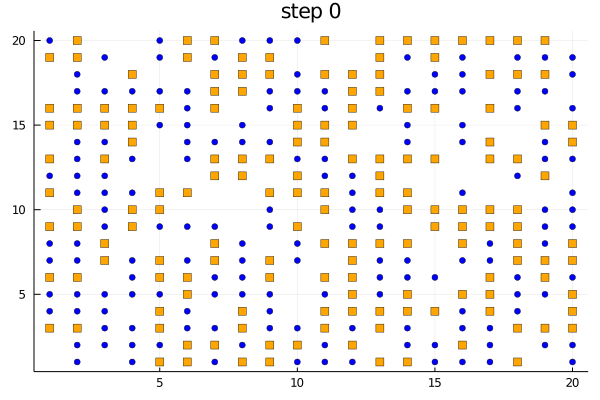
Visualizing the data
We can use the plotabm function to plot the distribution of agents on a 2D grid at every generation. Let's color the two groups orange and blue and make one a square and the other a circle.
groupcolor(a) = a.group == 1 ? :blue : :orange
groupmarker(a) = a.group == 1 ? :circle : :square
plotabm(model; ac = groupcolor, am = groupmarker, as = 4)
Animating the evolution
The function plotabm can be used to make your own animations
model = initialize();
anim = @animate for i in 0:10
    p1 = plotabm(model; ac = groupcolor, am = groupmarker, as = 4)
    title!(p1, "step $(i)")
    step!(model, agent_step!, 1)
end

gif(anim, "schelling.gif", fps = 2)
Replicates and parallel computing
We can run replicates of a simulation and collect all of them in a single DataFrame. To that end, we only need to specify replicates in the run! function:
model = initialize(numagents = 370, griddims = (20, 20), min_to_be_happy = 3)
data, _ = run!(model, agent_step!, 5; adata = adata, replicates = 3)
data[(end - 10):end, :]| step | sum_mood | maximum_x | replicate | |
|---|---|---|---|---|
| Int64 | Int64 | Int64 | Int64 | |
| 1 | 1 | 272 | 20 | 2 |
| 2 | 2 | 325 | 20 | 2 |
| 3 | 3 | 346 | 20 | 2 |
| 4 | 4 | 359 | 20 | 2 |
| 5 | 5 | 361 | 20 | 2 |
| 6 | 0 | 0 | 20 | 3 |
| 7 | 1 | 275 | 20 | 3 |
| 8 | 2 | 331 | 20 | 3 |
| 9 | 3 | 353 | 20 | 3 |
| 10 | 4 | 361 | 20 | 3 |
| 11 | 5 | 366 | 20 | 3 |
It is possible to run the replicates in parallel. For that, we should start julia with julia -p n where is the number of processing cores. Alternatively, we can define the number of cores from within a Julia session:
using Distributed
addprocs(4)
For distributed computing to work, all definitions must be preceded with @everywhere, e.g.
@everywhere using Agents
@everywhere mutable struct SchellingAgent ...
Then we can tell the run! function to run replicates in parallel:
data, _ = run!(model, agent_step!, 2, adata=adata,
               replicates=5, parallel=true)
Scanning parameter ranges
We often are interested in the effect of different parameters on the behavior of an agent-based model. Agents.jl provides the function paramscan to automatically explore the effect of different parameter values.
We have already defined our model initialization function as initialize. We now also define a processing function, that returns the percentage of happy agents:
happyperc(moods) = count(x -> x == true, moods) / length(moods)
adata = [(:mood, happyperc)]

parameters = Dict(
    :min_to_be_happy => collect(2:5), # expanded
    :numagents => [200, 300],         # expanded
    :griddims => (20, 20),            # not Vector = not expanded
)

data, _ = paramscan(parameters, initialize; adata = adata, n = 3, agent_step! = agent_step!)
data| step | happyperc_mood | min_to_be_happy | numagents | |
|---|---|---|---|---|
| Int64 | Float64 | Int64 | Int64 | |
| 1 | 0 | 0.0 | 2 | 200 |
| 2 | 1 | 0.645 | 2 | 200 |
| 3 | 2 | 0.89 | 2 | 200 |
| 4 | 3 | 0.97 | 2 | 200 |
| 5 | 0 | 0.0 | 3 | 200 |
| 6 | 1 | 0.365 | 3 | 200 |
| 7 | 2 | 0.635 | 3 | 200 |
| 8 | 3 | 0.74 | 3 | 200 |
| 9 | 0 | 0.0 | 4 | 200 |
| 10 | 1 | 0.165 | 4 | 200 |
| 11 | 2 | 0.31 | 4 | 200 |
| 12 | 3 | 0.365 | 4 | 200 |
| 13 | 0 | 0.0 | 5 | 200 |
| 14 | 1 | 0.02 | 5 | 200 |
| 15 | 2 | 0.05 | 5 | 200 |
| 16 | 3 | 0.065 | 5 | 200 |
| 17 | 0 | 0.0 | 2 | 300 |
| 18 | 1 | 0.82 | 2 | 300 |
| 19 | 2 | 0.95 | 2 | 300 |
| 20 | 3 | 0.97 | 2 | 300 |
| 21 | 0 | 0.0 | 3 | 300 |
| 22 | 1 | 0.626667 | 3 | 300 |
| 23 | 2 | 0.836667 | 3 | 300 |
| 24 | 3 | 0.923333 | 3 | 300 |
| 25 | 0 | 0.0 | 4 | 300 |
| 26 | 1 | 0.353333 | 4 | 300 |
| 27 | 2 | 0.553333 | 4 | 300 |
| 28 | 3 | 0.716667 | 4 | 300 |
| 29 | 0 | 0.0 | 5 | 300 |
| 30 | 1 | 0.153333 | 5 | 300 |
| 31 | 2 | 0.29 | 5 | 300 |
| 32 | 3 | 0.39 | 5 | 300 |
paramscan also allows running replicates per parameter setting:
data, _ = paramscan(
    parameters,
    initialize;
    adata = adata,
    n = 3,
    agent_step! = agent_step!,
    replicates = 3,
)

data[(end - 10):end, :]| step | happyperc_mood | replicate | min_to_be_happy | numagents | |
|---|---|---|---|---|---|
| Int64 | Float64 | Int64 | Int64 | Int64 | |
| 1 | 1 | 0.11 | 1 | 5 | 300 |
| 2 | 2 | 0.21 | 1 | 5 | 300 |
| 3 | 3 | 0.336667 | 1 | 5 | 300 |
| 4 | 0 | 0.0 | 2 | 5 | 300 |
| 5 | 1 | 0.173333 | 2 | 5 | 300 |
| 6 | 2 | 0.33 | 2 | 5 | 300 |
| 7 | 3 | 0.473333 | 2 | 5 | 300 |
| 8 | 0 | 0.0 | 3 | 5 | 300 |
| 9 | 1 | 0.193333 | 3 | 5 | 300 |
| 10 | 2 | 0.353333 | 3 | 5 | 300 |
| 11 | 3 | 0.42 | 3 | 5 | 300 |
We can combine all replicates with an aggregating function, such as mean, using the groupby and combine functions from the DataFrames package:
using DataFrames: groupby, combine, Not, select!
using Statistics: mean
gd = groupby(data,[:step, :min_to_be_happy, :numagents])
data_mean = combine(gd,[:happyperc_mood,:replicate] .=> mean)

select!(data_mean, Not(:replicate_mean))| step | min_to_be_happy | numagents | happyperc_mood_mean | |
|---|---|---|---|---|
| Int64 | Int64 | Int64 | Float64 | |
| 1 | 0 | 2 | 200 | 0.0 |
| 2 | 1 | 2 | 200 | 0.646667 |
| 3 | 2 | 2 | 200 | 0.843333 |
| 4 | 3 | 2 | 200 | 0.916667 |
| 5 | 0 | 3 | 200 | 0.0 |
| 6 | 1 | 3 | 200 | 0.291667 |
| 7 | 2 | 3 | 200 | 0.535 |
| 8 | 3 | 3 | 200 | 0.663333 |
| 9 | 0 | 4 | 200 | 0.0 |
| 10 | 1 | 4 | 200 | 0.12 |
| 11 | 2 | 4 | 200 | 0.305 |
| 12 | 3 | 4 | 200 | 0.398333 |
| 13 | 0 | 5 | 200 | 0.0 |
| 14 | 1 | 5 | 200 | 0.0266667 |
| 15 | 2 | 5 | 200 | 0.0616667 |
| 16 | 3 | 5 | 200 | 0.105 |
| 17 | 0 | 2 | 300 | 0.0 |
| 18 | 1 | 2 | 300 | 0.853333 |
| 19 | 2 | 2 | 300 | 0.961111 |
| 20 | 3 | 2 | 300 | 0.982222 |
| 21 | 0 | 3 | 300 | 0.0 |
| 22 | 1 | 3 | 300 | 0.584444 |
| 23 | 2 | 3 | 300 | 0.803333 |
| 24 | 3 | 3 | 300 | 0.892222 |
| 25 | 0 | 4 | 300 | 0.0 |
| 26 | 1 | 4 | 300 | 0.395556 |
| 27 | 2 | 4 | 300 | 0.634444 |
| 28 | 3 | 4 | 300 | 0.74 |
| 29 | 0 | 5 | 300 | 0.0 |
| 30 | 1 | 5 | 300 | 0.158889 |
| 31 | 2 | 5 | 300 | 0.297778 |
| 32 | 3 | 5 | 300 | 0.41 |
Note that the second argument takes the column names on which to split the data, i.e., it denotes which columns should not be aggregated. It should include the :step column and any parameter that changes among simulations. But it should not include the :replicate column. So in principle what we are doing here is simply averaging our result across the replicates.
Launching the interactive application
Given the definitions we have already created for a normal study of the Schelling model, it is almost trivial to launch an interactive application for it. First, we load InteractiveDynamics to access abm_data_exploration
using InteractiveDynamics
using GLMakie # we choose OpenGL as plotting backend
Then, we define a dictionary that maps some model-level parameters to a range of potential values, so that we can interactively change them.
parange = Dict(:min_to_be_happy => 0:8)Dict{Symbol,UnitRange{Int64}} with 1 entry:
:min_to_be_happy => 0:8Due to the different plotting backend (Plots.jl vs Makie.jl) we redefine some of the plotting functions (in the near future this won't be necessary, as everything will be Makie.jl based)
groupcolor(a) = a.group == 1 ? :blue : :orange
groupmarker(a) = a.group == 1 ? :circle : :rect
groupmarker (generic function with 1 method)
We define the alabels so that we can simple see the plotted timeseries with a shorter name (since the defaults can get large)
adata = [(:mood, sum), (x, mean)]
alabels = ["happy", "avg. x"]

model = initialize(; numagents = 300) # fresh model, noone happy
AgentBasedModel with 300 agents of type SchellingAgent space: GridSpace with size (20, 20), metric=chebyshev and periodic=false scheduler: random_activation properties: Dict(:min_to_be_happy => 3)
scene, adf, modeldf =
abm_data_exploration(model, agent_step!, dummystep, parange;
                ac = groupcolor, am = groupmarker, as = 1,
                adata = adata, alabels = alabels)