Attractors.jl Tutorial

Attractors is a component of the DynamicalSystems.jl library. This tutorial will walk you through its main functionality. That is, given a DynamicalSystem instance, find all its attractors and their basins of attraction. Then, continue these attractors, and their stability properties, across a parameter value. It also offers various functions that compute nonlocal stability properties for an attractor, any of which can be used in the continuation to quantify stability.

Besides this main functionality, there are plenty of other stuff, like for example edgestate or basins_fractal_dimension, but we won't cover anything else in this introductory tutorial. See the examples page instead.

Package versions used

import Pkg

Pkg.status(["Attractors", "CairoMakie", "OrdinaryDiffEqVerner"])

Status `~/work/Attractors.jl/Attractors.jl/docs/Project.toml`
  [f3fd9213] Attractors v2.0.3 `~/work/Attractors.jl/Attractors.jl`
  [13f3f980] CairoMakie v0.15.13
  [79d7bb75] OrdinaryDiffEqVerner v2.2.2

Tutorial - copy-pasteable version

Gotta go fast!

using Attractors, CairoMakie, OrdinaryDiffEqVerner
## Define key input: a `DynamicalSystem`
function modified_lorenz_rule(u, p, t)
    x, y, z = u; a, b = p
    dx = y - x
    dy = - x*z + b*abs(z)
    dz = x*y - a
    return SVector(dx, dy, dz)
end
p0 = [5.0, 0.1] # parameters
u0 = [-4.0, 5, 0] # state
diffeq = (alg = Vern9(), abstol = 1e-9, reltol = 1e-9, dt = 0.01) # solver options
ds = CoupledODEs(modified_lorenz_rule, u0, p0; diffeq)

## Define key input: a `BasinMap` that maps initial
## conditions to attractors of a `DynamicalSystem`
grid = (
    range(-15.0, 15.0; length = 150), # x
    range(-20.0, 20.0; length = 150), # y
    range(-20.0, 20.0; length = 150), # z
)
bmap = BasinMapRecurrences(ds, grid;
    consecutive_recurrences = 1000,
    consecutive_lost_steps = 100,
)

## Find attractors and their basins of attraction state space fraction
## by randomly sampling initial conditions in state sapce
sampler = RandomICsSampler(1000, grid)
fs = basins_fractions(bmap, sampler)
attractors = extract_attractors(bmap)

## found two attractors: one is a limit cycle, the other is chaotic
## visualize them
plot_attractors(attractors)

## continue all attractors and their basin fractions across any arbigrary
## curve in parameter space using a global continuation algorithm
algo = AttractorSeedContinueMatch(bmap)
ellipsoid(θ) = [1 => 5 + 0.5cos(θ), 2 => 0.1 + 0.01sin(θ)]
angles = range(0, 2π; length = 101)
pcurve = ellipsoid.(angles)
gcoutput = global_continuation(algo, pcurve, sampler)

## and visualize the results
fractions_cont = gcoutput.fractions
attractors_cont = gcoutput.attractors
fig = plot_basins_attractors_curves(
	fractions_cont, attractors_cont, A -> minimum(A[:, 1]), angles
)

Input: a `DynamicalSystem`

The key input for most functionality of Attractors.jl is an instance of a DynamicalSystem. If you don't know how to make a DynamicalSystem, you need to consult the main tutorial of the DynamicalSystems.jl library. For this tutorial we will use a modified Lorenz-like system with equations

\[\begin{align*} \dot{x} & = y - x \\ \dot{y} &= -x*z + b*|z| \\ \dot{z} &= x*y - a \\ \end{align*}\]

which we define in code as

using Attractors # part of `DynamicalSystems`, so it re-exports functionality for making them!
using OrdinaryDiffEqVerner # for accessing advanced ODE Solvers

function modified_lorenz_rule(u, p, t)
    x, y, z = u; a, b = p
    dx = y - x
    dy = - x * z + b * abs(z)
    dz = x * y - a
    return SVector(dx, dy, dz)
end

p0 = [5.0, 0.1] # parameters
u0 = [-4.0, 5, 0] # state
diffeq = (alg = Vern9(), abstol = 1.0e-9, reltol = 1.0e-9, dt = 0.01) # solver options
ds = CoupledODEs(modified_lorenz_rule, u0, p0; diffeq)

3-dimensional CoupledODEs
 deterministic: true
 discrete time: false
 in-place:      false
 dynamic rule:  modified_lorenz_rule
 ODE solver:    Vern9
 ODE kwargs:    (abstol = 1.0e-9, reltol = 1.0e-9, dt = 0.01)
 parameters:    [5.0, 0.1]
 time:          0.0
 state:         [-4.0, 5.0, 0.0]

Finding attractors and basins (basin map)

In this tutorial we will utilize two methods for finding attractors and their basins. Explanation of how they work is in their respective docs.

You can consult (Datseris et al., 2023) for a comparison between the two.

As far as the user is concerned, both algorithms are part of the same interface that is called BasinMap, as these constructs are mapping initial conditions to their corresponding basins of attraction. Thus, they are used the same way. The interface is extendable as well.

First, we create an instance of a BasinMap. For example, BasinMapRecurrences requires a tesselated grid of the state space to search for attractors in. It also allows the user to tune some meta parameters, but in our example they are already tuned for the dynamical system at hand. So we initialize

grid = (
    range(-10.0, 10.0; length = 150), # x
    range(-15.0, 15.0; length = 150), # y
    range(-15.0, 15.0; length = 150), # z
)

bmap = BasinMapRecurrences(
    ds, grid;
    consecutive_recurrences = 1000, attractor_locate_steps = 1000,
    consecutive_lost_steps = 100,
)

BasinMapRecurrences
 system:      CoupledODEs
 grid:        (-10.0:0.1342281879194631:10.0, -15.0:0.20134228187919462:15.0, -15.0:0.20134228187919462:15.0)
 attractors:  Dict{Int64, StateSpaceSet{3, Float64, SVector{3, Float64}}}()

This bmap can map any initial condition to tis corresponding basin, enumerated by unique integers. For example

bmap([-4.0, 5, 0])

while

bmap([4.0, 2, 0])

the fact that these two different initial conditions got assigned different IDs means that they converged to a different attractor under this basin map. Indeed,

bmap([1.0, 3, 2])

gets the same ID as the first initial condition.

This functionality is already incredibly powerful! To our knowledge the DynamicalSystems.jl library is the only dynamical systems software (in any language) that provides such an infrastructure for mapping initial conditions of any arbitrary dynamical system to its unique basins. And this is only the tip of this iceberg! The rest of the functionality of Attractors.jl is all full of brand new cutting edge progress in dynamical systems research.

Okay, back to the tutorial now! The found attractors are stored in the basin map internally, to obtain them we use the function

attractors = extract_attractors(bmap)

Dict{Int64, StateSpaceSet{3, Float64, SVector{3, Float64}}} with 2 entries:
  2 => 3-dimensional StateSpaceSet{Float64} with 320 points
  1 => 3-dimensional StateSpaceSet{Float64} with 935 points

In Attractors.jl, all information regarding attractors is always a standard Julia Dict, which maps attractor IDs (positive integers) to the corresponding quantity. Here the quantity are the attractors themselves, represented as StateSpaceSet.

We can visualize them with the convenience plotting function

using CairoMakie
plot_attractors(attractors)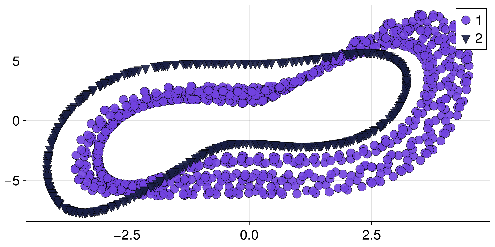

(this convenience function is a simple loop over scattering the values of the attractors dictionary)

In our example system we see that for the chosen parameters there are two coexisting attractors: a limit cycle and a chaotic attractor. There may be more attractors though! We've only checked a few initial conditions. However, it can get tedious to manually iterate over initial conditions, which is why this bmap is typically given to higher level functions for finding attractors and their basins of attraction. The simplest one is basins_fractions. Using the bmap, it finds "all" attractors of the dynamical system and reports the state space fraction each attractors attracts. The search is probabilistic, so "all" attractors means those that at least one initial condition converged to.

How initial conditions are sampled is described by the InitialConditionsSampelr super type and associated subtypes. One can prescribe a set vector of ICs, or randomly sample. This is what we will do here, but randomly sampling ICs within the grid.

sampler = RandomICsSampler(1000, grid) # sample 1000 ICs

RandomICsSampler{StateSpaceSets.RectangleGenerator{Float64, SVector{3, Float64}, Random.Xoshiro}}(StateSpaceSets.RectangleGenerator{Float64, SVector{3, Float64}, Random.Xoshiro}([-10.0, -15.0, -15.0], [20.0, 30.0, 30.0], [[0.0, 0.0, 0.0]], Random.Xoshiro(0xeaa184810311a250, 0x9c17f222a7b4e616, 0x07b2b061730c723a, 0xdff635e7c109d052, 0x0522462680b341f2)), 1000)

and finally call

fs = basins_fractions(bmap, sampler)

Dict{Int64, Float64} with 2 entries:
  2 => 0.349
  1 => 0.651

The returned fs is a dictionary mapping each attractor ID to the fraction of the state space the corresponding basin occupies. With this we can confirm that there are (likely) only two attractors and that both attractors are robust as both have sufficiently large basin fractions.

To obtain the full basins, which is computationally much more expensive, use basins_of_attraction.

Different Basin Map

Attractors.jl utilizes composable interfaces throughout its functionality. In the above example we used one particular method to find attractors, via recurrences in the state space. An alternative is BasinMapFeaturizeGroup.

For this method, we need to provide a "featurizing" function that given an trajectory (which is likely an attractor), it returns some features that will hopefully distinguish different attractors in a subsequent grouping step. Finding good features is typically a trial-and-error process, but for our system we already have some good features:

using Statistics: mean

function featurizer(A, t) # t is the time vector associated with trajectory A
    xmin = minimum(A[:, 1])
    ycen = mean(A[:, 2])
    return SVector(xmin, ycen)
end

featurizer (generic function with 1 method)

from which we initialize

bmap_fg = BasinMapFeaturizeGroup(ds, featurizer; Δt = 0.1)

BasinMapFeaturizeGroup
 system:      CoupledODEs
 Ttr:         100.0
 Δt:          0.1
 T:           100.0
 group via:   GroupViaClustering
 featurizer:  featurizer

BasinMapFeaturizeGroup allows for a third input, which is a "grouping configuration", that dictates how features will be grouped into attractors, as features are extracted from (randomly) sampled state space trajectories. In this tutorial we leave it at its default value, which is clustering using the DBSCAN algorithm. The keyword arguments are meta parameters which control how long to integrate each initial condition for, and what sampling time, to produce a trajectory A given to the featurizer function. Because one of the two attractors is chaotic, we need denser sampling time than the default.

We can use bmap_fg exactly as bmap:

fs2 = basins_fractions(bmap_fg, sampler)

attractors_fg = extract_attractors(bmap_fg)

plot_attractors(attractors_fg)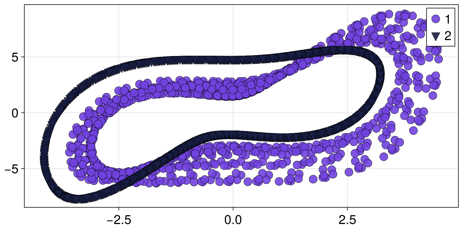

This basin map also found the attractors, but we should warn you: this basin map is less robust than BasinMapRecurrences. One of the reasons for this is that BasinMapFeaturizeGroup is not auto-terminating. For example, if we do not have enough transient integration time, the two attractors will get confused into one:

bmap_fg2 = BasinMapFeaturizeGroup(ds, featurizer; Ttr = 10, Δt = 0.1)
basins_fractions(bmap_fg2, sampler)
attractors_fg2 = extract_attractors(bmap_fg2)
plot_attractors(attractors_fg2)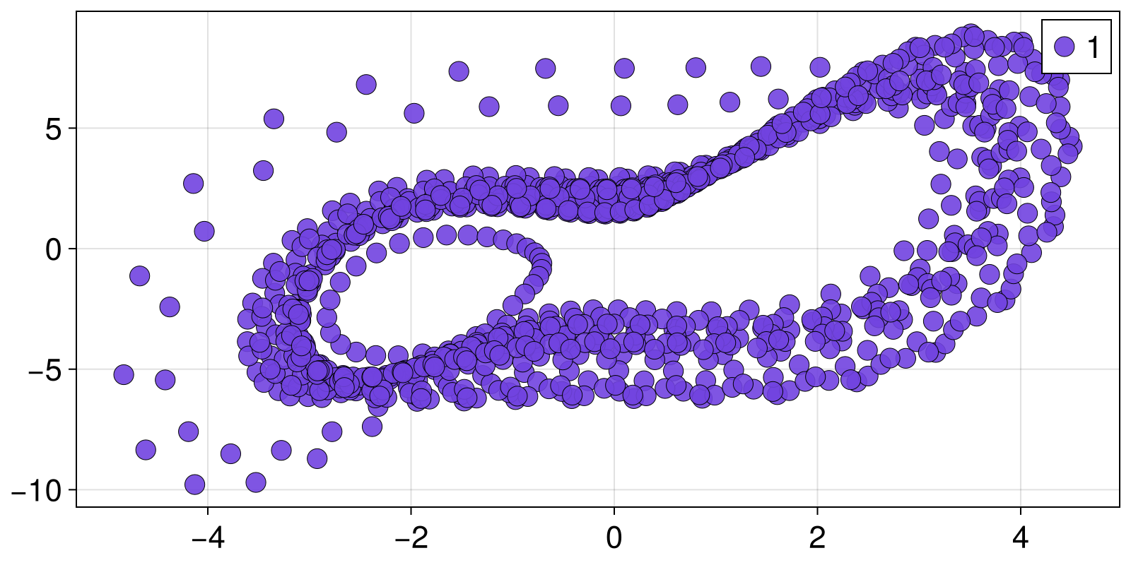

On the other hand, the downside of BasinMapRecurrences is that it can take quite a while to converge for chaotic or high dimensional systems.

Global continuation

If you have heard before the word "continuation", then you are likely aware of the traditional continuation-based bifurcation analysis (CBA) offered by many software, such as AUTO, CoCo, and in Julia BifurcationKit.jl. These software perform local continuation. Here we offer a completely different kind of continuation called global continuation. For an extensive comparison of the two, see our paper (Datseris et al., 2026) or have a look at the last paragraph in this tutorial. From our article:

!!! "quote" Global continuation finds and continues in parallel (practically) all system attractors and their response to finite perturbations by synthesising information from the whole state space, while placing a focus on the qualities or observables of a dynamical system that the practitioner cares about in context.

Because all attractors are simultaneously tracked across the parameter axis, the user may arbitrarily estimate any property of the attractors and how it varies as the parameter varies.

To perform a global continuation is surprisingly simple and requires only three clear inputs. First, we need to decide the global continuation algorithm which also references a BasinMap. In this example we will re-use the bmap to create the "flagship product" of Attractors.jl which is the general AttractorSeedContinueMatch. This algorithm uses the bmap to find all attractors at each parameter value and from the found attractors it continues them along a parameter axis using a seeding process (see its documentation string). Then, it performs a "matching" step, ensuring a "continuity" of the attractor label across the parameter axis. For now we ignore the matching step, leaving it to the default value. We'll use the bmap we created above and define

ascm = AttractorSeedContinueMatch(bmap)

AttractorSeedContinueMatch{BasinMapRecurrences{CoupledODEs{false, 3, OrdinaryDiffEqCore.ODEIntegrator{OrdinaryDiffEqVerner.Vern9{typeof(OrdinaryDiffEqCore.trivial_limiter!), typeof(OrdinaryDiffEqCore.trivial_limiter!), FastBroadcast.Serial, Val{true}}, false, SVector{3, Float64}, Nothing, Float64, Vector{Float64}, Float64, Float64, Vector{SVector{3, Float64}}, SciMLBase.ODESolution{Float64, 2, Vector{SVector{3, Float64}}, Nothing, Nothing, Vector{Float64}, Vector{Vector{SVector{3, Float64}}}, Nothing, SciMLBase.ODEProblem{SVector{3, Float64}, Tuple{Float64, Float64}, false, Vector{Float64}, SciMLBase.ODEFunction{false, SciMLBase.AutoSpecialize, typeof(Main.modified_lorenz_rule), LinearAlgebra.UniformScaling{Bool}, Nothing, Nothing, Nothing, Nothing, Nothing, Nothing, Nothing, Nothing, Nothing, Nothing, Nothing, Nothing, typeof(SciMLBase.DEFAULT_OBSERVED), Nothing, Nothing, Nothing, Nothing}, Base.Pairs{Symbol, Union{}, Tuple{}, @NamedTuple{}}, SciMLBase.StandardODEProblem}, OrdinaryDiffEqVerner.Vern9{typeof(OrdinaryDiffEqCore.trivial_limiter!), typeof(OrdinaryDiffEqCore.trivial_limiter!), FastBroadcast.Serial, Val{true}}, OrdinaryDiffEqCore.InterpolationData{SciMLBase.ODEFunction{false, SciMLBase.AutoSpecialize, typeof(Main.modified_lorenz_rule), LinearAlgebra.UniformScaling{Bool}, Nothing, Nothing, Nothing, Nothing, Nothing, Nothing, Nothing, Nothing, Nothing, Nothing, Nothing, Nothing, typeof(SciMLBase.DEFAULT_OBSERVED), Nothing, Nothing, Nothing, Nothing}, Vector{SVector{3, Float64}}, Vector{Float64}, Vector{Vector{SVector{3, Float64}}}, Nothing, OrdinaryDiffEqVerner.Vern9ConstantCache{Val{true}}, Nothing}, SciMLBase.DEStats, Nothing, Nothing, Nothing, Nothing}, SciMLBase.ODEFunction{false, SciMLBase.AutoSpecialize, typeof(Main.modified_lorenz_rule), LinearAlgebra.UniformScaling{Bool}, Nothing, Nothing, Nothing, Nothing, Nothing, Nothing, Nothing, Nothing, Nothing, Nothing, Nothing, Nothing, typeof(SciMLBase.DEFAULT_OBSERVED), Nothing, Nothing, Nothing, Nothing}, OrdinaryDiffEqVerner.Vern9ConstantCache{Val{true}}, OrdinaryDiffEqCore.DEOptions{Float64, Float64, Float64, Float64, typeof(DiffEqBase.ODE_DEFAULT_NORM), typeof(LinearAlgebra.opnorm), Bool, SciMLBase.CallbackSet{Tuple{}, Tuple{}}, typeof(DiffEqBase.ODE_DEFAULT_ISOUTOFDOMAIN), typeof(DiffEqBase.ODE_DEFAULT_PROG_MESSAGE), typeof(DiffEqBase.ODE_DEFAULT_UNSTABLE_CHECK), BinaryHeaps.BinaryHeap{Float64, BinaryHeaps.FasterForward}, BinaryHeaps.BinaryHeap{Float64, BinaryHeaps.FasterForward}, Nothing, Nothing, Float64, Tuple{}, Tuple{}, Tuple{}, DiffEqBase.DEVerbosity{true, SciMLLogging.Minimal, SciMLLogging.Minimal}, Nothing, typeof(OrdinaryDiffEqCore.trivial_limiter!), typeof(OrdinaryDiffEqCore.trivial_limiter!)}, SVector{3, Float64}, Float64, Nothing, DiffEqBase.DefaultInit, Nothing, OrdinaryDiffEqCore.PIControllerCache{Float64, Float64, SciMLBase.IntervalNonlinearProblem}, Random.TaskLocalRNG, Nothing, Nothing, Nothing, Nothing, Nothing, Nothing}, Vector{Float64}}, Attractors.BasinsInfo{3, Float64, Attractors.SparseArray{Int64, 3}, ArrayBasinsOfAttraction{Int64, 3, Attractors.SparseArray{Int64, 3}, Attractors.RegularGrid{3, StepRangeLen{Float64, Base.TwicePrecision{Float64}, Base.TwicePrecision{Float64}, Int64}}, Int64, StateSpaceSet{3, Float64, SVector{3, Float64}}}}, Attractors.RegularGrid{3, StepRangeLen{Float64, Base.TwicePrecision{Float64}, Base.TwicePrecision{Float64}, Int64}}, Base.Pairs{Symbol, Int64, Tuple{Symbol, Symbol, Symbol}, @NamedTuple{consecutive_recurrences::Int64, attractor_locate_steps::Int64, consecutive_lost_steps::Int64}}}, MatchBySSSetDistance{Centroid{Euclidean}, Float64}, typeof(Attractors._default_seeding)}(BasinMapRecurrences
 system:      CoupledODEs
 grid:        (-10.0:0.1342281879194631:10.0, -15.0:0.20134228187919462:15.0, -15.0:0.20134228187919462:15.0)
 attractors:  Dict{Int64, StateSpaceSet{3, Float64, SVector{3, Float64}}}(2 => 3-dimensional StateSpaceSet{Float64} with 320 points, 1 => 3-dimensional StateSpaceSet{Float64} with 935 points)
, MatchBySSSetDistance{Centroid{Euclidean}, Float64}(Centroid{Euclidean}(Euclidean(0.0)), Inf, false), Attractors._default_seeding)

The second input to global continuation is what parameter, and what values of that parameter, to continue over:

prange = 4.5:0.01:6
pidx = 1 # index of the parameter

Global continuation occurs over a prescribed parameter curve, so we convert this to

pcurve = [Dict(pidx => p) for p in prange]

151-element Vector{Dict{Int64, Float64}}:
 Dict(1 => 4.5)
 Dict(1 => 4.51)
 Dict(1 => 4.52)
 Dict(1 => 4.53)
 Dict(1 => 4.54)
 Dict(1 => 4.55)
 Dict(1 => 4.56)
 Dict(1 => 4.57)
 Dict(1 => 4.58)
 Dict(1 => 4.59)
 ⋮
 Dict(1 => 5.92)
 Dict(1 => 5.93)
 Dict(1 => 5.94)
 Dict(1 => 5.95)
 Dict(1 => 5.96)
 Dict(1 => 5.97)
 Dict(1 => 5.98)
 Dict(1 => 5.99)
 Dict(1 => 6.0)

Then, the third and final input is how, and how densely, to sample the state space. Here we re-use the sampler from before. So we can now call:

gco = global_continuation(ascm, pcurve, sampler)

GlobalContinuationOutput with fields:
 attractors
 fractions
 quantifiers
 other
 pcurve

This normally takes about a minute of compute depending on your computer. The output is GlobalContinuationOutput which can contain a variety of information but always contains the following two crucial pieces of information given as two vectors:

fractions_cont = gco.fractions
attractors_cont = gco.attractors;

Each vector is a dictionary mapping basin IDs to their basin fractions, or their state space sets, respectively. Both vectors have the same size as the parameter axis. For example, the attractors at the 77-th parameter value are:

attractors_cont[77]

Dict{Int64, StateSpaceSet{3, Float64, SVector{3, Float64}}} with 2 entries:
  2 => 3-dimensional StateSpaceSet{Float64} with 843 points
  1 => 3-dimensional StateSpaceSet{Float64} with 325 points

If you want to transform the output to the alternative format of a dictionary of vectors, use continuation_series. There is also a fantastic convenience function for animating the attractors evolution, that utilizes things we have already defined:

animate_attractors_continuation(ds, gco)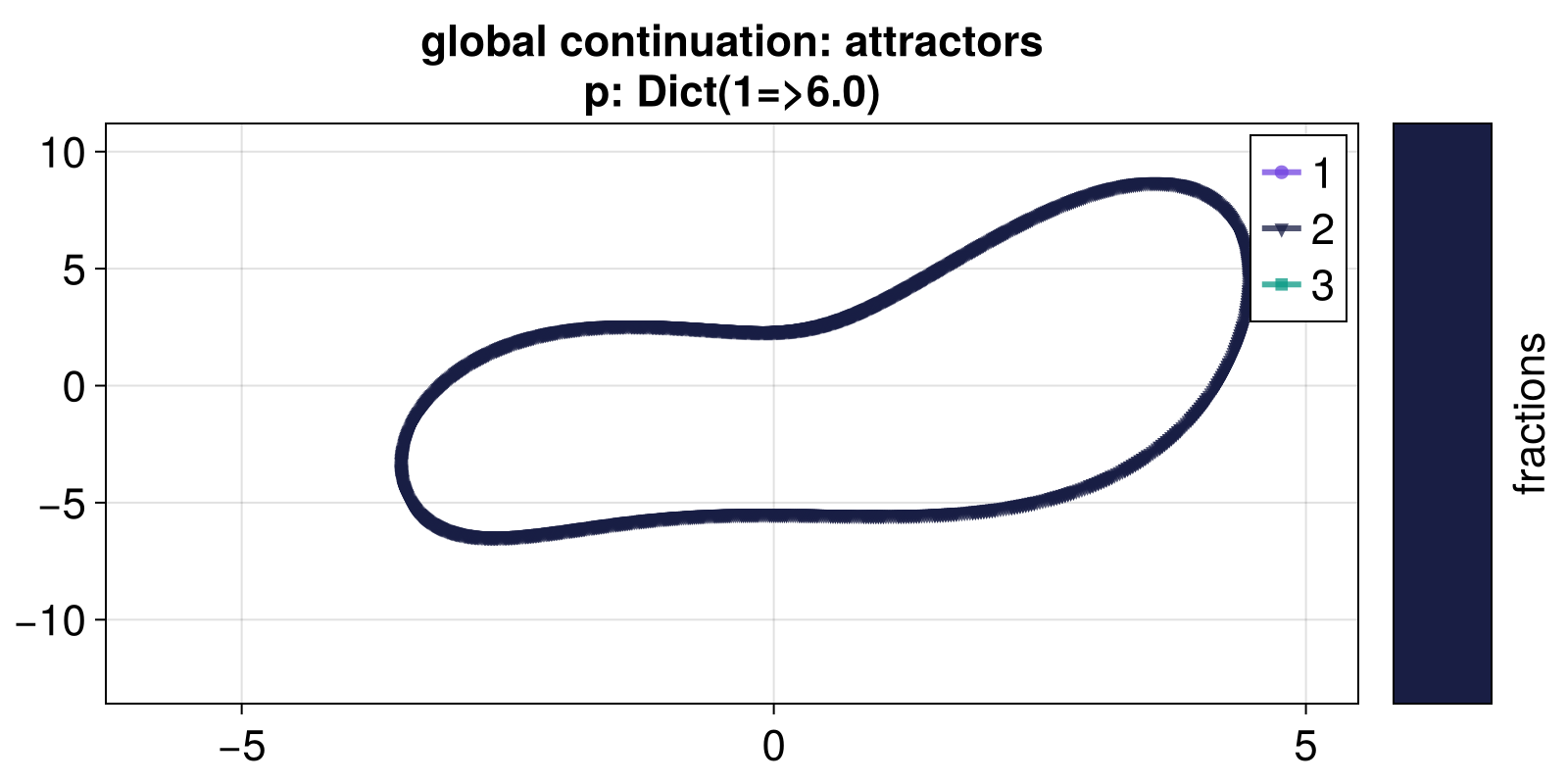

Hah, how cool is that! The attractors pop in and out of existence like out of nowhere! It can be difficult to find these attractors in traditional continuation software where a rough estimate of the period is required!

Now typically a continuation is visualized in a 2D plot where the x axis is the parameter axis. We can do this with the convenience function:

fig = plot_basins_attractors_curves(
    fractions_cont, attractors_cont, A -> minimum(A[:, 1]), prange,
)

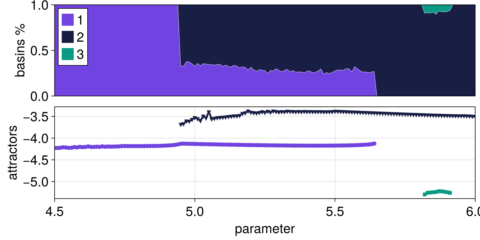
In the top panel are the basin fractions, by default plotted as stacked bars. Bottom panel is a visualization of some feature(s) of the tracked attractors. The argument A -> minimum(A[:, 1]) is a function that maps an attractor into a real number for plotting. A vector of such functions can be given instead.

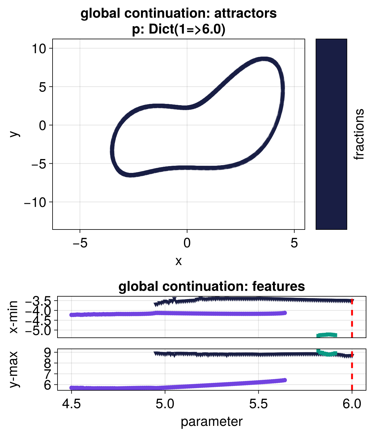
Moreover, you can combine the animation we created above with this continuation plot so you can see both the attractors in state space as well as some chosen feature(s). This is done by calling animate_attractors_continuation again with additional keyword arguments like so:

fig = animate_attractors_continuation(
    ds, gco;
    figure = (size = (600, 700),),
    axis = (ylabel = "y", xlabel = "x"),
    savename = "globalcont_extra.mp4",
    add_legend = false,
    a2rs = [A -> minimum(A[:, 1]), A -> maximum(A[:, 2])],
    a2rs_ylabels = ["x-min", "y-max"],
    a2rs_ratio = 0.33,
    vline_kwargs = (linestyle = :dash, linewidth = 3, color = "red"),
    prange,
)

Different matching procedures

By default attractors are matched by their distance in state space. The default matcher is MatchBySSSetDistance, and is given implicitly as a default 2nd argument when creating AttractorSeedContinueMatch. But like anything else in Attractors.jl, "matchers" also follow a well-defined and extendable interface, see IDMatchers for that.

Let's say that the default matching that we chose above isn't desirable. For example, one may argue that the attractor that pops up at the end of the continuation should have been assigned the same ID as attractor 1, because they are both to the left (see the video above). In reality one wouldn't really request that, because looking the video of attractors above shows that the attractors labelled "1", "2", and "3" are all completely different. But we argue here for example that "3" should have been the same as "1".

Thankfully during a global continuation the "matching" step is completely separated from the "finding and continuing" step. If we don't like the initial matching, we can call match_sequentially! with a new instance of a matcher, and match again, without having to recompute the attractors and their basin fractions. For example, using this matcher:

matcher = MatchBySSSetDistance(use_vanished = true)

MatchBySSSetDistance{Centroid{Euclidean}, Float64}(Centroid{Euclidean}(Euclidean(0.0)), Inf, true)

will compare a new attractor with the latest instance of attractors with a given ID that have ever existed, irrespectively if they exist in the current parameter or not. This means, that the attractor "3" would in fact be compared with both attractor "2" and "1", even if "1" doesn't exist in the parameter "3" started existing at. And because "3" is closer to "1" than to "2", it will get matched to attractor "1" and get the same ID.

Let's see this in action:

attractors_cont2 = deepcopy(attractors_cont)

match_sequentially!(attractors_cont2, matcher)

fig = plot_attractors_curves(
    attractors_cont2, A -> minimum(A[:, 1]), prange,
)

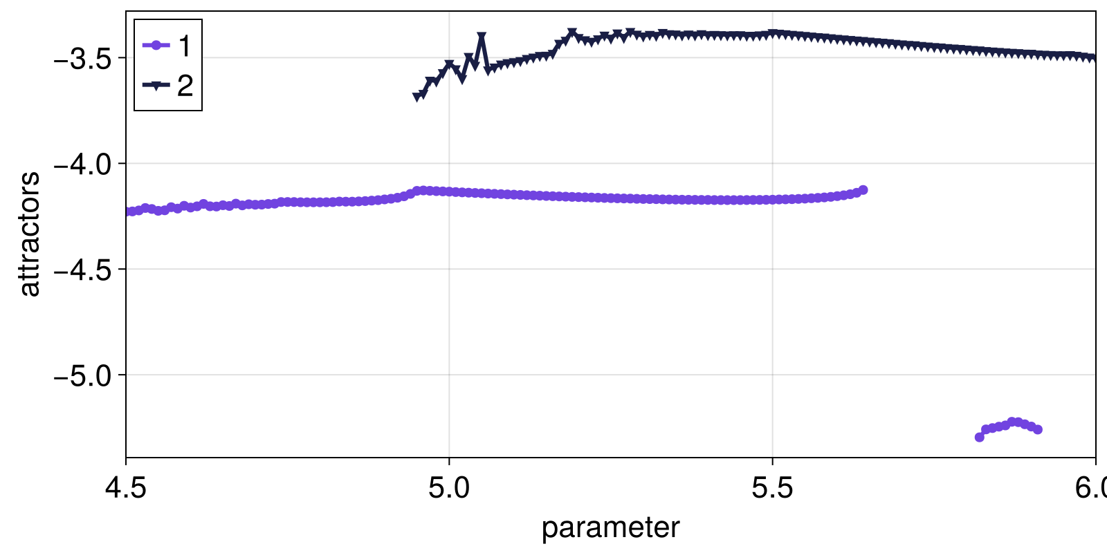
and as we can see, the new attractor at the end of the parameter range got assigned the same ID as the original attractor "1". For more ways of matching attractors see IDMatcher.

Continuation along arbitrary parameter curves

One of the many advantages of the global continuation is that we can choose what parameters to continue over. We can provide any arbitrary curve in parameter space. This is possible because (1) finding and matching attractors are two completely orthogonal steps, and (2) it is completely fine for attractors to dissapear (and perhaps re-appear) during a global continuation.

For example, we can probe an elipsoid defined as

ellipsoid(θ) = [1 => 5 + 0.5cos(θ), 2 => 0.1 + 0.01sin(θ)]
θs = range(0, 2π; length = 101)
pcurve = ellipsoid.(θs)

101-element Vector{Vector{Pair{Int64, Float64}}}:
 [1 => 5.5, 2 => 0.1]
 [1 => 5.499013364214136, 2 => 0.10062790519529313]
 [1 => 5.496057350657239, 2 => 0.10125333233564304]
 [1 => 5.491143625364344, 2 => 0.10187381314585725]
 [1 => 5.4842915805643155, 2 => 0.10248689887164855]
 [1 => 5.475528258147577, 2 => 0.10309016994374948]
 [1 => 5.4648882429441255, 2 => 0.10368124552684678]
 [1 => 5.45241352623301, 2 => 0.10425779291565074]
 [1 => 5.438153340021932, 2 => 0.10481753674101715]
 [1 => 5.422163962751007, 2 => 0.10535826794978997]
 ⋮
 [1 => 5.438153340021932, 2 => 0.09518246325898286]
 [1 => 5.45241352623301, 2 => 0.09574220708434927]
 [1 => 5.4648882429441255, 2 => 0.09631875447315323]
 [1 => 5.475528258147577, 2 => 0.09690983005625053]
 [1 => 5.4842915805643155, 2 => 0.09751310112835145]
 [1 => 5.491143625364344, 2 => 0.09812618685414276]
 [1 => 5.496057350657239, 2 => 0.09874666766435695]
 [1 => 5.499013364214136, 2 => 0.09937209480470688]
 [1 => 5.5, 2 => 0.1]

here each component maps the parameter index to its value. We can just give this pcurve to the global continuation, using the same basin map and continuation algorithm, but adjusting the matching process so that vanished attractors are kept in "memory"

matcher = MatchBySSSetDistance(use_vanished = true)

ascm = AttractorSeedContinueMatch(bmap, matcher)

gco = global_continuation(ascm, pcurve, sampler)
attractors_cont = gco.attractors

101-element Vector{Dict{Int64, StateSpaceSet{3, Float64, SVector{3, Float64}}}}:
 Dict(2 => 3-dimensional StateSpaceSet{Float64} with 332 points, 1 => 3-dimensional StateSpaceSet{Float64} with 519 points)
 Dict(2 => 3-dimensional StateSpaceSet{Float64} with 313 points, 1 => 3-dimensional StateSpaceSet{Float64} with 510 points)
 Dict(2 => 3-dimensional StateSpaceSet{Float64} with 314 points, 1 => 3-dimensional StateSpaceSet{Float64} with 557 points)
 Dict(2 => 3-dimensional StateSpaceSet{Float64} with 327 points, 1 => 3-dimensional StateSpaceSet{Float64} with 589 points)
 Dict(2 => 3-dimensional StateSpaceSet{Float64} with 338 points, 1 => 3-dimensional StateSpaceSet{Float64} with 604 points)
 Dict(2 => 3-dimensional StateSpaceSet{Float64} with 307 points, 1 => 3-dimensional StateSpaceSet{Float64} with 637 points)
 Dict(2 => 3-dimensional StateSpaceSet{Float64} with 341 points, 1 => 3-dimensional StateSpaceSet{Float64} with 610 points)
 Dict(2 => 3-dimensional StateSpaceSet{Float64} with 329 points, 1 => 3-dimensional StateSpaceSet{Float64} with 660 points)
 Dict(2 => 3-dimensional StateSpaceSet{Float64} with 313 points, 1 => 3-dimensional StateSpaceSet{Float64} with 630 points)
 Dict(2 => 3-dimensional StateSpaceSet{Float64} with 320 points, 1 => 3-dimensional StateSpaceSet{Float64} with 665 points)
 ⋮
 Dict(2 => 3-dimensional StateSpaceSet{Float64} with 305 points, 1 => 3-dimensional StateSpaceSet{Float64} with 654 points)
 Dict(2 => 3-dimensional StateSpaceSet{Float64} with 344 points, 1 => 3-dimensional StateSpaceSet{Float64} with 609 points)
 Dict(2 => 3-dimensional StateSpaceSet{Float64} with 316 points, 1 => 3-dimensional StateSpaceSet{Float64} with 623 points)
 Dict(2 => 3-dimensional StateSpaceSet{Float64} with 347 points, 1 => 3-dimensional StateSpaceSet{Float64} with 583 points)
 Dict(2 => 3-dimensional StateSpaceSet{Float64} with 323 points, 1 => 3-dimensional StateSpaceSet{Float64} with 543 points)
 Dict(2 => 3-dimensional StateSpaceSet{Float64} with 323 points, 1 => 3-dimensional StateSpaceSet{Float64} with 492 points)
 Dict(2 => 3-dimensional StateSpaceSet{Float64} with 320 points, 1 => 3-dimensional StateSpaceSet{Float64} with 495 points)
 Dict(2 => 3-dimensional StateSpaceSet{Float64} with 316 points, 1 => 3-dimensional StateSpaceSet{Float64} with 515 points)
 Dict(2 => 3-dimensional StateSpaceSet{Float64} with 315 points, 1 => 3-dimensional StateSpaceSet{Float64} with 534 points)

and animate the result

animate_attractors_continuation(ds, gco; savename = "curvecont.mp4");

Enhancing the continuation with more stability quantifiers or other quantities

The standard stability quantifier that is reported during a global continuation is the basin fractions. This is primarily because it is computed automatically as we find the different attractors. There are many more stability quantifiers that could be more useful in different contexts. Attractors.jl offers the unique possibility of estimating a multitude of known quantifiers of stability in the literature of dynamical systems during a single global continuation pass. This is done with the StabilityQuantifiersAccumulator data structure. You can visit its documentation string to learn about all different stability quantifiers. If you find some stability quantifiers not included in the StabilityQuantifiersAccumulator then either open an Issue and tell us about it or even better make a Pull Request and contribute it yourself!

Using StabilityQuantifiersAccumulator is very easy. If you have already performed a global continuation then you can utilize the function stability_quantifiers_along_continuation to run through it again and estimate now all stability quantifiers.

result = stability_quantifiers_along_continuation(
    ds, attractors_cont, pcurve, sampler; ε = 0.1
)
keys(result)

KeySet for a Dict{String, Vector{Dict{Int64, Float64}}} with 19 entries. Keys:
  "characteristic_return_time"
  "maximal_amplification_time"
  "finite_time_basin_stability"
  "mean_noncritical_shock_magnitude"
  "median_convergence_pace"
  "reactivity"
  "basin_stability"
  "maximal_convergence_pace"
  "mean_convergence_pace"
  "basin_fraction"
  "minimal_critical_shock_magnitude"
  "maximal_noncritical_shock_magnitude"
  "boundary_basin_entropy"
  "mean_convergence_time"
  "basin_entropy"
  "median_convergence_time"
  "maximal_convergence_time"
  "maximal_amplification"
  "intermingledness1"

The result is a dictionary mapping the stability quantifier name (as a string) to the continuation of the quantifier. We can see there are quite a lot of quantifiers that have been estimated! So the values of result are the same type as the fractions_cont we have computed before. This means it is straightforward to visualize these new stability quantifiers. For example, let's say we want to visualize

chosen = ["median_convergence_pace", "minimal_critical_shock_magnitude"]
abbrev = ["MCP", "MCS"]

2-element Vector{String}:
 "MCP"
 "MCS"

then we just use the visualization function plot_continuation_curves

ukeys = unique_keys(attractors_cont) # so that we ignore key -1 (divergent orbits)
fig = plot_attractors_curves(attractors_cont, A -> minimum(A[:, 1]), θs)
for (i, c) in enumerate(chosen)
    ax = Axis(fig[1 - i, 1]; ylabel = abbrev[i])
    quantifier_cont = result[c]
    plot_continuation_curves!(ax, quantifier_cont, θs; ukeys, add_legend = false)
    hidexdecorations!(ax; grid = false)
end
resize!(fig, 600, 500)
fig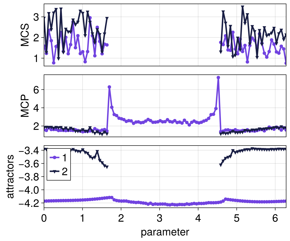

For more specialization on estimating these stability quantifiers, see the documentation of StabilityQuantifiersAccumulator.

One of the biggest strengths of Attractors.jl is that it is not an isolated software. It is part of DynamicalSystems.jl. We can straightforwardly use any other functionality of the library to enhance this continuation, even beyond stability quantifiers. Let's also estimate and visualize the maximum Lyapunov exponent for each attractor. We first import the function that estimates the MLE

using ChaosTools: lyapunov

and then, the estimation itself is rather simple:

lis = map(enumerate(pcurve)) do (i, p) # loop over parameters
    set_parameters!(ds, p) # important! We use the dynamical system!
    attractors = attractors_cont[i]
    # Return a dictionary mapping attractor IDs to their MLE
    Dict(k => lyapunov(ds, 10000.0; u0 = A[1]) for (k, A) in attractors)
end

101-element Vector{Dict{Int64, Float64}}:
 Dict(2 => 0.00019091471377764683, 1 => -0.0002119913632783521)
 Dict(2 => 0.00014980463189935247, 1 => 0.00040511902992282193)
 Dict(2 => 7.476665716587241e-5, 1 => 5.424696072148014e-5)
 Dict(2 => 2.1960075319157012e-5, 1 => 0.00012498136246759045)
 Dict(2 => -4.446104555732576e-6, 1 => 0.00028378943802262306)
 Dict(2 => 0.00024249351382641478, 1 => 0.0001650763131363472)
 Dict(2 => -3.8971285192317404e-5, 1 => 0.00015241615988700134)
 Dict(2 => 0.00014262023771758622, 1 => 0.00011274215594985475)
 Dict(2 => 0.00022681021125479304, 1 => -4.549952167348434e-5)
 Dict(2 => 0.00016672311518385155, 1 => 0.00015377374488858428)
 ⋮
 Dict(2 => -6.729619788765758e-5, 1 => -6.7280424124118316e-6)
 Dict(2 => 7.063951541035724e-5, 1 => 6.609577079854288e-5)
 Dict(2 => -3.766446431474381e-5, 1 => 0.0002805675971083807)
 Dict(2 => 9.769353484931321e-5, 1 => 0.0001366441263614784)
 Dict(2 => 6.664539979093824e-5, 1 => 0.00013987466027227572)
 Dict(2 => 0.00022939932908840968, 1 => -5.8477588879070586e-6)
 Dict(2 => 0.0001686565793237196, 1 => 0.00012084045999035551)
 Dict(2 => 0.00012948070022355946, 1 => 0.00013765382472620118)
 Dict(2 => 0.0001532707212462886, 1 => -0.0001968847980835667)

The above map loop may be intimidating if you are a beginner, but it is really just a shorter way to write a for loop for our example. We iterate over all parameters, and for each we first update the dynamical system with the correct parameter, and then extract the MLE for each attractor. map just means that we don't have to pre-allocate a new vector before the loop; it creates it for us.

Notice: in the example here we we computed the Lyapunov exponents after the fact. We could do it however duing the first-pass of the continuation of the StabilityQuantifiersAccumulator by providing the extras argument to it, see e.g., the example of additional quantifiers online.

Regardless, we now visualize the MLE with the same way as any other quantity over the continuation:

axλ = Axis(fig[-length(chosen), 1]; ylabel = "MLE")
hidexdecorations!(axλ)
plot_continuation_curves!(axλ, lis, θs; add_legend = false)
fig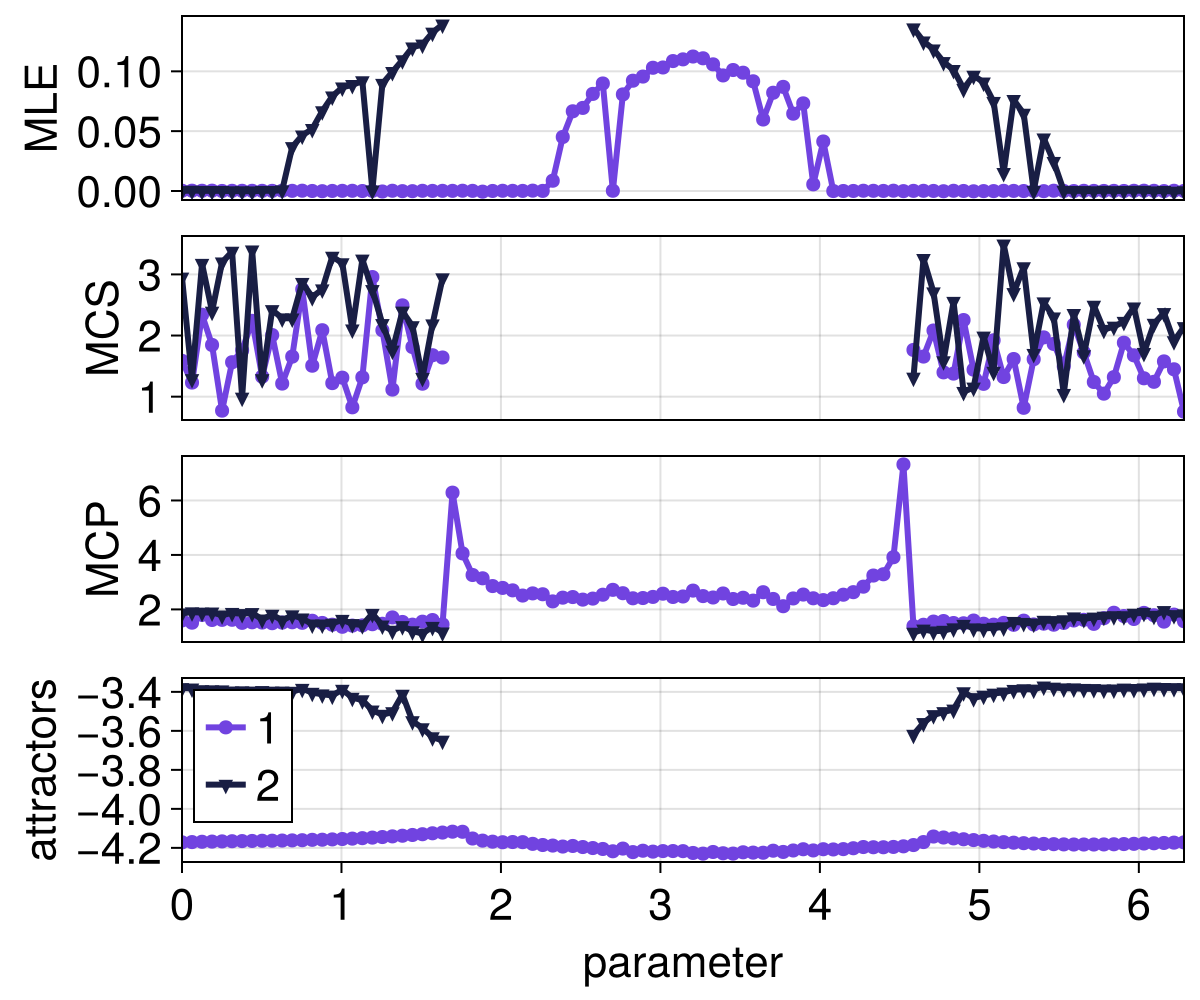

This reveals crucial information for tha attractors, whether they are chaotic or not, that we would otherwise obtain only by visualizing the system dynamics at every single point in the continuation parameter.

Multiparameter continuation

For global continuation, there is truthfully no difference between single and multiple parameter continuation. To efficiently cover a multidimensional parameter space, We provide the convenience function hilbert_pcurve. Let's use it here to continue over both parameters

specs = Dict(1 => (5, 6, 2^4), 2 => (0.1, 0.2, 2^4))
pcurve = hilbert_pcurve(specs)

256-element Vector{Dict{Int64, Float64}}:
 Dict(2 => 0.1, 1 => 5.0)
 Dict(2 => 0.10666666666666667, 1 => 5.0)
 Dict(2 => 0.10666666666666667, 1 => 5.066666666666666)
 Dict(2 => 0.1, 1 => 5.066666666666666)
 Dict(2 => 0.1, 1 => 5.133333333333334)
 Dict(2 => 0.1, 1 => 5.2)
 Dict(2 => 0.10666666666666667, 1 => 5.2)
 Dict(2 => 0.10666666666666667, 1 => 5.133333333333334)
 Dict(2 => 0.11333333333333333, 1 => 5.133333333333334)
 Dict(2 => 0.11333333333333333, 1 => 5.2)
 ⋮
 Dict(2 => 0.18666666666666668, 1 => 5.133333333333334)
 Dict(2 => 0.19333333333333333, 1 => 5.133333333333334)
 Dict(2 => 0.19333333333333333, 1 => 5.2)
 Dict(2 => 0.2, 1 => 5.2)
 Dict(2 => 0.2, 1 => 5.133333333333334)
 Dict(2 => 0.2, 1 => 5.066666666666666)
 Dict(2 => 0.19333333333333333, 1 => 5.066666666666666)
 Dict(2 => 0.19333333333333333, 1 => 5.0)
 Dict(2 => 0.2, 1 => 5.0)

We need to add a threshold to the continuation matching. Here we'll add an arbitrary value, but in a research setup this would need to be studied. Thankfully, the matching can be redone after the continuation at practically no cost using match_sequentially!.

matcher = MatchBySSSetDistance(use_vanished = true, threshold = 0.5)
ascm = AttractorSeedContinueMatch(bmap, matcher)

AttractorSeedContinueMatch{BasinMapRecurrences{CoupledODEs{false, 3, OrdinaryDiffEqCore.ODEIntegrator{OrdinaryDiffEqVerner.Vern9{typeof(OrdinaryDiffEqCore.trivial_limiter!), typeof(OrdinaryDiffEqCore.trivial_limiter!), FastBroadcast.Serial, Val{true}}, false, SVector{3, Float64}, Nothing, Float64, Vector{Float64}, Float64, Float64, Vector{SVector{3, Float64}}, SciMLBase.ODESolution{Float64, 2, Vector{SVector{3, Float64}}, Nothing, Nothing, Vector{Float64}, Vector{Vector{SVector{3, Float64}}}, Nothing, SciMLBase.ODEProblem{SVector{3, Float64}, Tuple{Float64, Float64}, false, Vector{Float64}, SciMLBase.ODEFunction{false, SciMLBase.AutoSpecialize, typeof(Main.modified_lorenz_rule), LinearAlgebra.UniformScaling{Bool}, Nothing, Nothing, Nothing, Nothing, Nothing, Nothing, Nothing, Nothing, Nothing, Nothing, Nothing, Nothing, typeof(SciMLBase.DEFAULT_OBSERVED), Nothing, Nothing, Nothing, Nothing}, Base.Pairs{Symbol, Union{}, Tuple{}, @NamedTuple{}}, SciMLBase.StandardODEProblem}, OrdinaryDiffEqVerner.Vern9{typeof(OrdinaryDiffEqCore.trivial_limiter!), typeof(OrdinaryDiffEqCore.trivial_limiter!), FastBroadcast.Serial, Val{true}}, OrdinaryDiffEqCore.InterpolationData{SciMLBase.ODEFunction{false, SciMLBase.AutoSpecialize, typeof(Main.modified_lorenz_rule), LinearAlgebra.UniformScaling{Bool}, Nothing, Nothing, Nothing, Nothing, Nothing, Nothing, Nothing, Nothing, Nothing, Nothing, Nothing, Nothing, typeof(SciMLBase.DEFAULT_OBSERVED), Nothing, Nothing, Nothing, Nothing}, Vector{SVector{3, Float64}}, Vector{Float64}, Vector{Vector{SVector{3, Float64}}}, Nothing, OrdinaryDiffEqVerner.Vern9ConstantCache{Val{true}}, Nothing}, SciMLBase.DEStats, Nothing, Nothing, Nothing, Nothing}, SciMLBase.ODEFunction{false, SciMLBase.AutoSpecialize, typeof(Main.modified_lorenz_rule), LinearAlgebra.UniformScaling{Bool}, Nothing, Nothing, Nothing, Nothing, Nothing, Nothing, Nothing, Nothing, Nothing, Nothing, Nothing, Nothing, typeof(SciMLBase.DEFAULT_OBSERVED), Nothing, Nothing, Nothing, Nothing}, OrdinaryDiffEqVerner.Vern9ConstantCache{Val{true}}, OrdinaryDiffEqCore.DEOptions{Float64, Float64, Float64, Float64, typeof(DiffEqBase.ODE_DEFAULT_NORM), typeof(LinearAlgebra.opnorm), Bool, SciMLBase.CallbackSet{Tuple{}, Tuple{}}, typeof(DiffEqBase.ODE_DEFAULT_ISOUTOFDOMAIN), typeof(DiffEqBase.ODE_DEFAULT_PROG_MESSAGE), typeof(DiffEqBase.ODE_DEFAULT_UNSTABLE_CHECK), BinaryHeaps.BinaryHeap{Float64, BinaryHeaps.FasterForward}, BinaryHeaps.BinaryHeap{Float64, BinaryHeaps.FasterForward}, Nothing, Nothing, Float64, Tuple{}, Tuple{}, Tuple{}, DiffEqBase.DEVerbosity{true, SciMLLogging.Minimal, SciMLLogging.Minimal}, Nothing, typeof(OrdinaryDiffEqCore.trivial_limiter!), typeof(OrdinaryDiffEqCore.trivial_limiter!)}, SVector{3, Float64}, Float64, Nothing, DiffEqBase.DefaultInit, Nothing, OrdinaryDiffEqCore.PIControllerCache{Float64, Float64, SciMLBase.IntervalNonlinearProblem}, Random.TaskLocalRNG, Nothing, Nothing, Nothing, Nothing, Nothing, Nothing}, Vector{Float64}}, Attractors.BasinsInfo{3, Float64, Attractors.SparseArray{Int64, 3}, ArrayBasinsOfAttraction{Int64, 3, Attractors.SparseArray{Int64, 3}, Attractors.RegularGrid{3, StepRangeLen{Float64, Base.TwicePrecision{Float64}, Base.TwicePrecision{Float64}, Int64}}, Int64, StateSpaceSet{3, Float64, SVector{3, Float64}}}}, Attractors.RegularGrid{3, StepRangeLen{Float64, Base.TwicePrecision{Float64}, Base.TwicePrecision{Float64}, Int64}}, Base.Pairs{Symbol, Int64, Tuple{Symbol, Symbol, Symbol}, @NamedTuple{consecutive_recurrences::Int64, attractor_locate_steps::Int64, consecutive_lost_steps::Int64}}}, MatchBySSSetDistance{Centroid{Euclidean}, Float64}, typeof(Attractors._default_seeding)}(BasinMapRecurrences
 system:      CoupledODEs
 grid:        (-10.0:0.1342281879194631:10.0, -15.0:0.20134228187919462:15.0, -15.0:0.20134228187919462:15.0)
 attractors:  Dict{Int64, StateSpaceSet{3, Float64, SVector{3, Float64}}}(2 => 3-dimensional StateSpaceSet{Float64} with 534 points, 1 => 3-dimensional StateSpaceSet{Float64} with 315 points)
, MatchBySSSetDistance{Centroid{Euclidean}, Float64}(Centroid{Euclidean}(Euclidean(0.0)), 0.5, true), Attractors._default_seeding)

and proceed as usual

fractions_cont, attractors_cont = global_continuation(ascm, pcurve, sampler)

GlobalContinuationOutput with fields:
 attractors
 fractions
 quantifiers
 other
 pcurve

The output is exactly of the same type, and as such very easy to post-process. For example, let's find all parameter values that support an attractor with x-minimum less than -5 (this is the teal attractor in the starting video of this page)

function find_condition(attractors::Dict)
    return any(A -> minimum(A[:, 1]) < -5, values(attractors))
end
pidxs = findall(find_condition, attractors_cont)

24-element Vector{Int64}:
  83
  84
  93
  94
  96
  97
  98
  99
 100
 109
   ⋮
 159
 160
 161
 162
 175
 176
 177
 180
 181

We can now scatterplot the parameters that have, or don't have, this property:

coords = [SVector(p[1], p[2]) for p in pcurve]
markers = [i ∈ pidxs ? :circle : :rect for i in eachindex(pcurve)]
colors = [i ∈ pidxs ? :black : :blue for i in eachindex(pcurve)]
fig, ax = scatter(coords; marker = markers, color = colors)
ax.xlabel = "parameter 1"
ax.ylabel = "parameter 2"
ax.title = "parameters that have teal attractor"
fig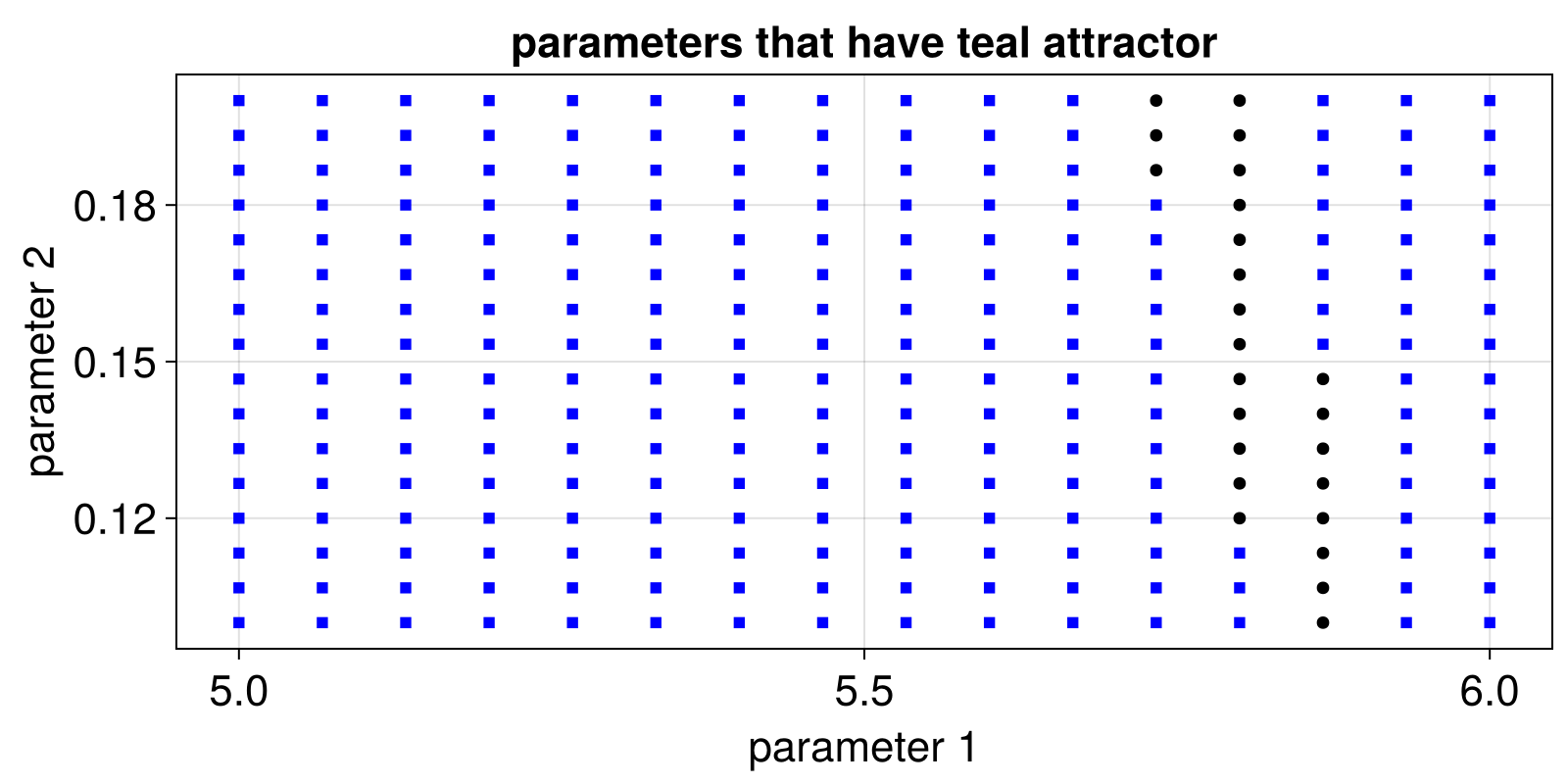

Conclusion and comparison with traditional local continuation

We've reached the end of the tutorial! Some aspects we haven't highlighted is how most of the infrastructure of Attractors.jl is fully extendable. You will see this when reading the documentation strings of key structures like BasinMap. All documentation strings are in the API page. See the examples page for more varied applications. And lastly, see the comparison page in our docs that attempts to do the same analysis of our Tutorial with traditional local continuation and bifurcation analysis software showing that (at least for this example) using Attractors.jl is clearly beneficial over the alternatives.