Lyapunov Exponents
Lyapunov exponents measure exponential rates of separation of nearby trajectories in the flow of a dynamical system. The concept of these exponents is best explained in Chapter 3 of Nonlinear Dynamics, Datseris & Parlitz, Springer 2022. The explanations of the chapter directly utilize the code of the functions in this page.
Lyapunov Spectrum
The function lyapunovspectrum calculates the entire spectrum of the Lyapunov exponents of a system:
ChaosTools.lyapunovspectrum — Function
lyapunovspectrum(ds::DynamicalSystem, N, k = dimension(ds); kwargs...) -> λsCalculate the spectrum of Lyapunov exponents [Lyapunov1992] of ds by applying a QR-decomposition on the parallelepiped defined by the deviation vectors, in total for N evolution steps. Return the spectrum sorted from maximum to minimum. The third argument k is optional, and dictates how many lyapunov exponents to calculate (defaults to dimension(ds)).
See also lyapunov, local_growth_rates.
Note: This function simply initializes a TangentDynamicalSystem and calls the method below. This means that the automatic Jacobian is used by default. Initialize manually a TangentDynamicalSystem if you have a hand-coded Jacobian.
Keyword arguments
u0 = current_state(ds): State to start from.Ttr = 0: Extra transient time to evolve the system before application of the algorithm. Should beIntfor discrete systems. Both the system and the deviation vectors are evolved for this time.Δt = 1: Time of individual evolutions between successive orthonormalization steps. For continuous systems this is approximate.show_progress = false: Display a progress bar of the process.
Description
The method we employ is "H2" of [Geist1990], originally stated in [Benettin1980], and explained in educational form in [DatserisParlitz2022].
The deviation vectors defining a D-dimensional parallelepiped in tangent space are evolved using the tangent dynamics of the system (see TangentDynamicalSystem). A QR-decomposition at each step yields the local growth rate for each dimension of the parallelepiped. At each step the parallelepiped is re-normalized to be orthonormal. The growth rates are then averaged over N successive steps, yielding the lyapunov exponent spectrum.
lyapunovspectrum(tands::TangentDynamicalSystem, N::Int; Ttr, Δt, show_progress)The low-level method that is called by lyapunovspectrum(ds::DynamicalSystem, ...). Use this method for looping over different initial conditions or parameters by calling reinit! to tands.
Also use this method if you have a hand-coded Jacobian to pass when creating tands.
Example
For example, the Lyapunov spectrum of the folded towel map is calculated as:
using ChaosTools
function towel_rule(x, p, n)
    @inbounds x1, x2, x3 = x[1], x[2], x[3]
    SVector( 3.8*x1*(1-x1) - 0.05*(x2+0.35)*(1-2*x3),
    0.1*( (x2+0.35)*(1-2*x3) - 1 )*(1 - 1.9*x1),
    3.78*x3*(1-x3)+0.2*x2 )
end
function towel_jacob(x, p, n)
    row1 = SVector(3.8*(1 - 2x[1]), -0.05*(1-2x[3]), 0.1*(x[2] + 0.35))
    row2 = SVector(-0.19((x[2] + 0.35)*(1-2x[3]) - 1),  0.1*(1-2x[3])*(1-1.9x[1]),  -0.2*(x[2] + 0.35)*(1-1.9x[1]))
    row3 = SVector(0.0,  0.2,  3.78(1-2x[3]))
    return vcat(row1', row2', row3')
end

ds = DeterministicIteratedMap(towel_rule, [0.085, -0.121, 0.075], nothing)
tands = TangentDynamicalSystem(ds; J = towel_jacob)

λλ = lyapunovspectrum(tands, 10000)
3-element Vector{Float64}:
0.43224475747701546
0.3722615352085776
-3.296655735650821lyapunovspectrum also works for continuous time systems and will auto-generate a Jacobian function if one is not give. For example,
function lorenz_rule(u, p, t)
    σ = p[1]; ρ = p[2]; β = p[3]
    du1 = σ*(u[2]-u[1])
    du2 = u[1]*(ρ-u[3]) - u[2]
    du3 = u[1]*u[2] - β*u[3]
    return SVector{3}(du1, du2, du3)
end

lor = CoupledODEs(lorenz_rule, fill(10.0, 3), [10, 32, 8/3])
λλ = lyapunovspectrum(lor, 10000; Δt = 0.1)
3-element Vector{Float64}:
0.984974201005527
0.0036498494900651193
-14.655223962016466lyapunovspectrum is also very fast:
using BenchmarkTools
ds = DeterministicIteratedMap(towel_rule, [0.085, -0.121, 0.075], nothing)
tands = TangentDynamicalSystem(ds; J = towel_jacob)

@btime lyapunovspectrum($tands, 10000)
966.500 μs (10 allocations: 576 bytes) # on my laptopHere is an example of using reinit! to iterate over different parameter values to compute the exponents over a given parameter range.
using ChaosTools, CairoMakie

henon_rule(x, p, n) = SVector{2}(1.0 - p[1]*x[1]^2 + x[2], p[2]*x[1])
henon_jacob(x, p, n) = SMatrix{2,2}(-2*p[1]*x[1], p[2], 1.0, 0.0)
ds = DeterministicIteratedMap(henon_rule, zeros(2), [1.4, 0.3])
tands = TangentDynamicalSystem(ds; J = henon_jacob)

as = 0.8:0.005:1.225;
λs = zeros(length(as), 2)

for i in eachindex(as)
    set_parameter!(ds, 1, as[i])
    λs[i, :] .= lyapunovspectrum(ds, 10000; Ttr = 500)
end

fig = Figure()
ax = Axis(fig[1,1]; xlabel = L"a", ylabel = L"\lambda")
for j in 1:2
    lines!(ax, as, λs[:, j])
end
fig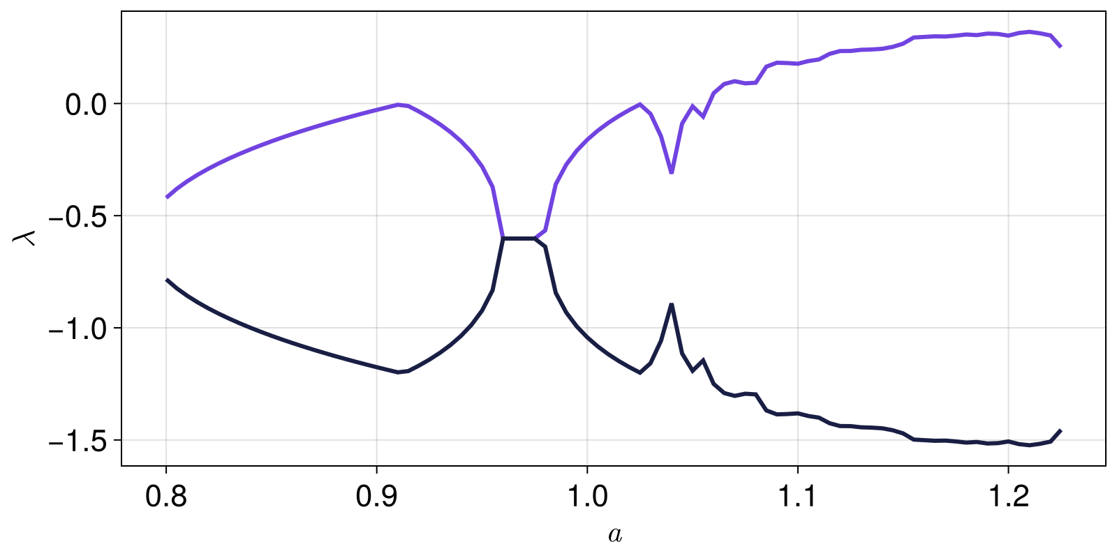
You can parallelize this code as well, see the main tutorial of DynamicalSystems.jl for an example.
Maximum Lyapunov Exponent
It is possible to get only the maximum Lyapunov exponent simply by giving 1 as the third argument of lyapunovspectrum. However, there is a second algorithm that calculates the maximum exponent:
ChaosTools.lyapunov — Function
lyapunov(ds::DynamicalSystem, Τ; kwargs...) -> λCalculate the maximum Lyapunov exponent λ using a method due to Benettin [Benettin1976], which simply evolves two neighboring trajectories (one called "given" and one called "test") while constantly rescaling the test one.
T denotes the total time of evolution (should be Int for discrete time systems).
See also lyapunovspectrum, local_growth_rates.
Keyword arguments
show_progress = false: Display a progress bar of the process.u0 = initial_state(ds): Initial condition.Ttr = 0: Extra "transient" time to evolve the trajectories before starting to measure the exponent. Should beIntfor discrete systems.d0 = 1e-9: Initial & rescaling distance between the two neighboring trajectories.d0_lower = 1e-3*d0: Lower distance threshold for rescaling.d0_upper = 1e+3*d0: Upper distance threshold for rescaling.Δt = 1: Time of evolution between each check rescaling of distance.inittest = (u1, d0) -> u1 .+ d0/sqrt(length(u1)): A function that given(u1, d0)initializes the test state with distanced0from the given stateu1(Dis the dimension of the system). This function can be used when you want to avoid the test state appearing in a region of the phase-space where it would have e.g. different energy or escape to infinity.
Description
Two neighboring trajectories with initial distance d0 are evolved in time. At time $t_i = t_{i-1} + \Delta t$, if their distance $d(t_i)$ either exceeds the d0_upper, or is lower than d0_lower, the test trajectory is rescaled back to having distance d0 from the reference one, while the rescaling keeps the difference vector along the maximal expansion/contraction direction: $u_2 \to u_1+(u_2−u_1)/(d(t_i)/d_0)$.
The maximum Lyapunov exponent is the average of the time-local Lyapunov exponents
\[\lambda = \frac{1}{t_{n} - t_0}\sum_{i=1}^{n} \ln\left( a_i \right),\quad a_i = \frac{d(t_{i})}{d_0}.\]
Performance notes
This function simply initializes a ParallelDynamicalSystem and calls the method below.
The reason we only conditionally rescale the neighboring trajectories is computational: the averaging will give correct result overall if the trajectories never diverge or converge (i.e., for periodic orbits).
lyapunov(pds::ParallelDynamicalSystem, T; Ttr, Δt, d0, d0_upper, d0_lower)The low-level method that is called by lyapunov(ds::DynamicalSystem, ...). Use this method for looping over different initial conditions or parameters by calling reinit! to pds.
For example:
using ChaosTools
henon_rule(x, p, n) = SVector{2}(1.0 - p[1]*x[1]^2 + x[2], p[2]*x[1])
henon = DeterministicIteratedMap(henon_rule, zeros(2), [1.4, 0.3])
λ = lyapunov(henon, 10000; d0 = 1e-7, d0_upper = 1e-4, Ttr = 100)0.42018736282059616The lyapunov function can return NaN in two cases: (1) if integration fails to converge at any time; and (2) if during rescaling, the initial distance $d_0$ is not in the interval $d_{0, \rm{lower}} \leq d_0 \leq d_{0, \rm{upper}}$. In both cases, a warning is displayed and you must check your integrator and dynamical system definition and parameters to ensure they fit the algorithm.
Local Growth Rates
ChaosTools.local_growth_rates — Function
local_growth_rates(ds::DynamicalSystem, points::StateSpaceSet; kwargs...) → λlocalCompute the local exponential growth rate(s) of perturbations of the dynamical system ds for initial conditions given in points. For each initial condition u ∈ points, S total perturbations are created and evolved exactly for time Δt. The exponential local growth rate is defined simply by log(g/g0)/Δt with g0 the initial perturbation size and g the size after Δt. Thus, λlocal is a matrix of size (length(points), S).
This function is a modification of lyapunov. It uses the full nonlinear dynamics and a ParallelDynamicalSystem to evolve the perturbations, but does not do any re-scaling, thus allowing probing state and time dependence of perturbation growth. The actual growth is given by exp(λlocal * Δt).
The output of this function is sometimes called "Nonlinear Local Lyapunov Exponent".
Keyword arguments
S = 100Δt = 5perturbation: If given, it should be a functionperturbation(ds, u, j)that outputs a perturbation vector (preferrablySVector) given the system, current initial conditionuand the counterj ∈ 1:S. If not given, a random perturbation is generated with norm given by the keyworde = 1e-6.
Here is a simple example using the Henon map
using ChaosTools
using Statistics, CairoMakie

henon_rule(x, p, n) = SVector{2}(1.0 - p[1]*x[1]^2 + x[2], p[2]*x[1])
he = DeterministicIteratedMap(henon_rule, zeros(2), [1.4, 0.3])
points = trajectory(he, 2000; Ttr = 100)[1]

λlocal = local_growth_rates(he, points; Δt = 1)

λmeans = mean(λlocal; dims = 2)
λstds = std(λlocal; dims = 2)
x, y = columns(points)
fig, ax, obj = scatter(x, y; color = vec(λmeans))
Colorbar(fig[1,2], obj)
fig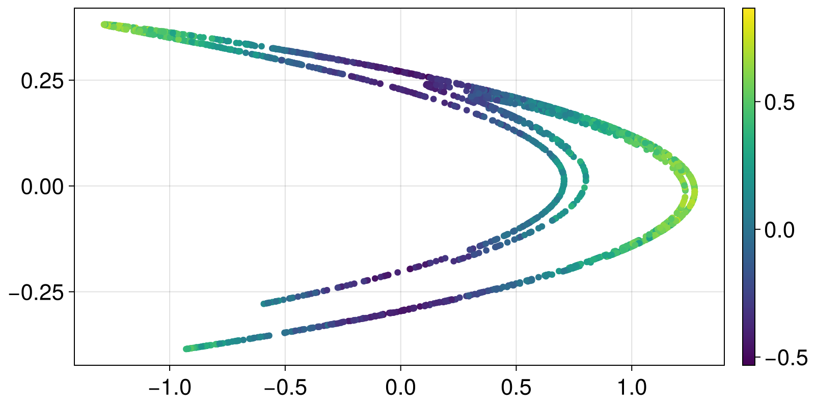
Lyapunov exponent from data
ChaosTools.lyapunov_from_data — Function
lyapunov_from_data(R::StateSpaceSet, ks; kwargs...)For the given dataset R, which is expected to represent a trajectory of a dynamical system, calculate and return E(k), which is the average logarithmic distance between states of a neighborhood that are evolved in time for k steps (k must be integer). The slope of E vs k approximates the maximum Lyapunov exponent.
Typically R is the result of delay coordinates embedding of a timeseries (see DelayEmbeddings.jl).
Keyword arguments
refstates = 1:(length(R) - ks[end]): Vector of indices that notes which states of the dataset should be used as "reference states", which means that the algorithm is applied for all state indices contained inrefstates.w::Int = 1: The Theiler window.ntype = NeighborNumber(1): The neighborhood type. EitherNeighborNumberorWithinRange. See Neighborhoods for more info.distance = FirstElement(): Specifies what kind of distance function is used in the logarithmic distance of nearby states. Allowed distances values areFirstElement()orEuclidean(), see below for more info. The metric for finding neighbors is always the Euclidean one.
Description
If the dataset exhibits exponential divergence of nearby states, then it should hold
\[E(k) \approx \lambda\cdot k \cdot \Delta t + E(0)\]
for a well defined region in the $k$ axis, where $\lambda$ is the approximated maximum Lyapunov exponent. $\Delta t$ is the time between samples in the original timeseries. You can use linear_region with arguments (ks .* Δt, E) to identify the slope (= $\lambda$) immediately, assuming you have chosen sufficiently good ks such that the linear scaling region is bigger than the saturated region.
The algorithm used in this function is due to Parlitz[Skokos2016], which itself expands upon Kantz[Kantz1994]. In sort, for each reference state a neighborhood is evaluated. Then, for each point in this neighborhood, the logarithmic distance between reference state and neighborhood state(s) is calculated as the "time" index k increases. The average of the above over all neighborhood states over all reference states is the returned result.
If the distance is Euclidean() then use the Euclidean distance of the full D-dimensional points (distance $d_E$ in ref.[Skokos2016]). If however the distance is FirstElement(), calculate the absolute distance of only the first elements of the points of R (distance $d_F$ in ref.[Skokos2016], useful when R comes from delay embedding).
Neighborhood.NeighborNumber — Type
NeighborNumber(k::Int) <: SearchTypeSearch type representing the k nearest neighbors of the query (or approximate neighbors, depending on the search structure).
Neighborhood.WithinRange — Type
WithinRange(r::Real) <: SearchTypeSearch type representing all neighbors with distance ≤ r from the query (according to the search structure's metric).
Let's apply the method to a timeseries from a continuous time system. In this case, one must be a bit more thoughtful when choosing parameters. The following example helps the users get familiar with the process:
using ChaosTools, CairoMakie

function lorenz_rule(u, p, t)
    σ = p[1]; ρ = p[2]; β = p[3]
    du1 = σ*(u[2]-u[1])
    du2 = u[1]*(ρ-u[3]) - u[2]
    du3 = u[1]*u[2] - β*u[3]
    return SVector{3}(du1, du2, du3)
end

ds = CoupledODEs(lorenz_rule, fill(10.0, 3), [10, 32, 8/3])
# create a timeseries of 1 dimension
Δt = 0.05
x = trajectory(ds, 1000.0; Ttr = 10, Δt)[1][:, 1]
20001-element Vector{Float64}:
4.080373151926001
4.240648215569559
4.9957366262635965
6.360963430437676
8.368663200858672
10.871010890922056
13.195165384996477
14.06894343005168
12.645851679172127
9.67435546664522
⋮
2.026571274062356
-0.5541100306065054
-2.0951960391652142
-3.23878245192252
-4.439640568914813
-6.012857404286814
-8.157203821460808
-10.82257043058155
-13.362239397504581From prior knowledge of the system, we know we need to use k up to about 150. However, due to the dense time sampling, we don't have to compute for every k in the range 0:150. Instead, we can use
ks = 0:4:1500:4:148Now we plot some example computations using delay embeddings to "reconstruct" the chaotic attractor
using DelayEmbeddings: embed
fig = Figure()
ax = Axis(fig[1,1]; xlabel="k (0.05×t)", ylabel="E - E(0)")
ntype = NeighborNumber(5) #5 nearest neighbors of each state

for d in [4, 8], τ in [7, 15]
    r = embed(x, d, τ)

    # E1 = lyapunov_from_data(r, ks1; ntype)
    # λ1 = ChaosTools.linreg(ks1 .* Δt, E1)[2]
    # plot(ks1,E1.-E1[1], label = "dense, d=$(d), τ=$(τ), λ=$(round(λ1, 3))")

    E2 = lyapunov_from_data(r, ks; ntype)
    λ2 = ChaosTools.linreg(ks .* Δt, E2)[2]
    lines!(ks, E2.-E2[1]; label = "d=$(d), τ=$(τ), λ=$(round(λ2, digits = 3))")
end
axislegend(ax; position = :lt)
ax.title = "Continuous Reconstruction Lyapunov"
fig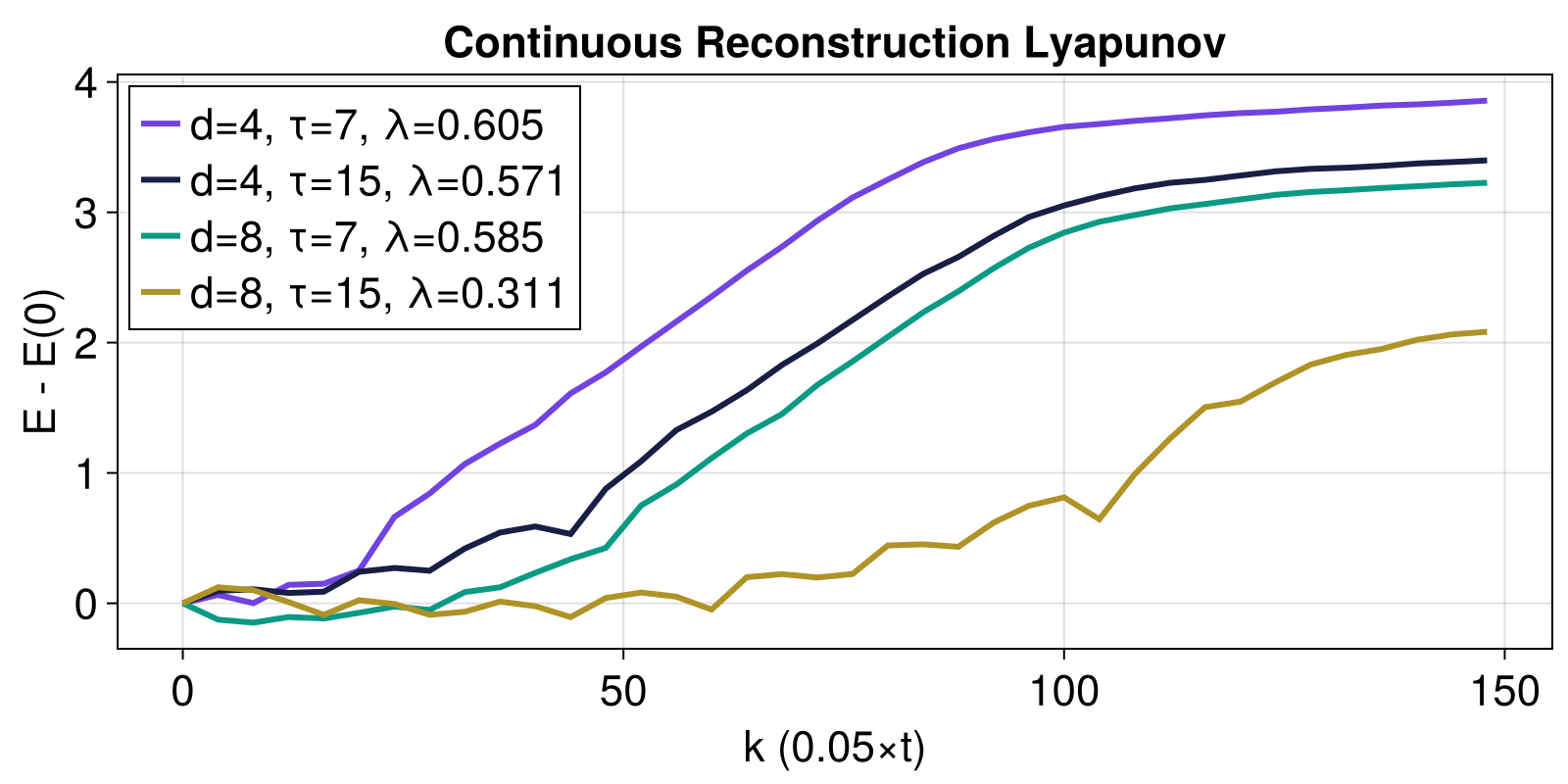
As you can see, using τ = 15 is not a great choice! The estimates with τ = 7 though are very good (the actual value is around λ ≈ 0.89...). Notice that above a linear regression was done over the whole curves, which doesn't make sense. One should identify a linear scaling region and extract the slope of that one. The function linear_region from FractalDimensions.jl does this!
Instantaneous Lyapunov exponent for non-autonomous systems
ChaosTools.ensemble_averaged_pairwise_distance — Function
ensemble_averaged_pairwise_distance(ds, init_states::StateSpaceSet, T, pidx;kwargs...) -> ρ,tCalculate the ensemble-averaged pairwise distance function ρ for non-autonomous dynamical systems with a time-dependent parameter, using the metod described by [^Jánosi,Tél2024]. Time-dependence is assumed to be a linear drift. The rate of change of the parameter needs to be stored in the parameter container of the system p = current_parameters(ds), at the index pidx. In case of autonomous systems (with no drift), pidx can be set to any index as a dummy. To every member of the ensemble init_states, a perturbed initial condition is assigned. ρ(t) is the natural log of state space distance between the original and perturbed states averaged over all pairs, calculated for all time steps up to T.
Keyword arguments
initial_params = deepcopy(current_parameters(ds)): initial parametersTtr = 0: transient time used to evolve initial states to reach initial autonomous attractor (without drift)perturbation = perturbation_normal: if given, it should be a functionperturbation(ds,ϵ), which outputs perturbed state vector ofds(preferrablySVector). If not given, a normally distributed random perturbation with normϵis added.Δt = 1: step sizeϵ = sqrt(dimension(ds))*1e-10: initial distance between pairs of original and perturbed initial conditions
Description
In non-autonomous systems with parameter drift, long time averages are less useful to assess chaoticity. Thus, quantities using time averages are rather calculated using ensemble averages. Here, a new quantity called the Ensemble-averaged pairwise distance (EAPD) is used to measure chaoticity of the snapshot attractor/ state space object traced out by the ensemble [JánosiTél2024].
To any member of the original ensemble (init_states) a close neighbour (test) is added at an initial distance ϵ. Quantity d(t) is the state space distance between a test particle and an ensemble member at time t . If init_states are randomly initialized (far from the attractor at the initial parameter), and there's no transient, the first few time steps cannot be used to calculate any reliable averages. The function of the EAPD ρ(t) is defined as the average logarithmic distance between original and perturbed initial conditions at every time step: ρ(t) = ⟨ln d(t)⟩
An analog of the classical largest Lyapunov exponent can be extracted from the EAPD function ρ: the local slope can be considered an instantaneous Lyapunov exponent.
Example
Example of a rate-dependent (linearly drifting parameter) system
#r parameter is replaced by r(n) = r0 + R*n drift term
function drifting_logistic(x,p,n)
    r0,R = p
    return SVector( (r0 + R*n)*x[1]*(1-x[1]) )
end

r0 = 3.8 #inital parameter
R = 0.001 #rate parameter
p = [r0,R] # pidx = 2

init_states = StateSpaceSet(rand(1000)) #initial states of the ensemble
ds = DeterministicIteratedMap(drifting_logistic, [0.1], p)
ρ,times = ensemble_averaged_pairwise_distance(ds,init_states,100,2;Ttr=1000)ChaosTools.lyapunov_instant — Function
lyapunov_instant(ρ,times;interval=1:length(times)) -> λ(t)Calculates the instantaneous Lyapunov exponent by taking the slope of the ensemble-averaged pairwise distance function ρ wrt. to the saved time points times in interval.
Let's see first if the ensemble approach is equivalent to the usual time-averaging case (Benettin algorithm) in the autonomous case. Here is a simple example using the Henon map:
henon_rule(x, p, n) = SVector{2}(1.0 - p[1]*x[1]^2 + x[2], p[2]*x[1])
ds = DeterministicIteratedMap(henon_rule, zeros(2), [1.4, 0.3, 0.0])

init_states = StateSpaceSet(0.2 .* rand(1000,2))
pidx = 3 # set to dummy, not used anywhere (no drift)
ρ,times = ensemble_averaged_pairwise_distance(ds,init_states,100,pidx;Ttr=5000)
λ_inst = lyapunov_instant(ρ,times;interval=20:30) #fit to middle part of the curve (slope is constant until saturation)
λ = lyapunov(ds,1000;Ttr=5000) #standard (Benettin) way
@show λ_inst, λ
(0.4264898173658178, 0.4130128860298917)Now look at the nonautonomous Duffing map with drifting ε parameter:
using CairoMakie
using ChaosTools

function duffing_drift(u0 = [0.1, 0.25]; ω = 1.0, β = 0.2, ε0 = 0.4, α=0.00045)
    return CoupledODEs(duffing_drift_rule, u0, [ω, β, ε0, α])
end

@inbounds function duffing_drift_rule(x, p, t)
    ω, β, ε0, α = p
    dx1 = x[2]
    dx2 = (ε0+α*t)*cos(ω*t) + x[1] - x[1]^3 - 2β * x[2]
    return SVector(dx1, dx2)
end

duffing = duffing_drift()
duffing_map = StroboscopicMap(duffing,2π)
init_states = randn(5000,2) #use an ensemble of 5000
pidx = 4 #ε is the fourth parameter
ρ,times = ensemble_averaged_pairwise_distance(duffing_map,StateSpaceSet(init_states),100,pidx;Ttr=20)

#measure slope of ρ at two places
λ_inst = lyapunov_instant(ρ,times;interval=5:10)
λ_inst2 = lyapunov_instant(ρ,times;interval=22:25)

fig,ax,obj = scatter(times, ρ,
    markersize = 6,
    color = :gray10,
    label = L"\omega = 1, \beta = 0.2, \epsilon_0 = 0.4, \alpha=0.00045",
    axis = (xlabel = L"t", ylabel = L"\rho(t)",xlabelsize = 20,ylabelsize = 20))

lines!(ax, times[5:10], ρ[5] .+ λ_inst*[0:5;], color = (:red, 0.7),linewidth = 3)
lines!(ax, times[22:25], ρ[22] .+ λ_inst2*[0:3;],color = (:red, 0.7), linewidth = 3)

text!(ax, times[5]+8, ρ[10],text = L"\lambda = %$(round(λ_inst;digits=3))",
color = :red,align = (:left, :center),fontsize = 18)

text!(ax, times[22]+8, ρ[24],text = L"\lambda = %$(round(λ_inst2;digits=3))",
color = :red, align = (:left, :center), fontsize = 18)

axislegend(ax, position = :rb, nbanks = 2,labelsize = 18)
fig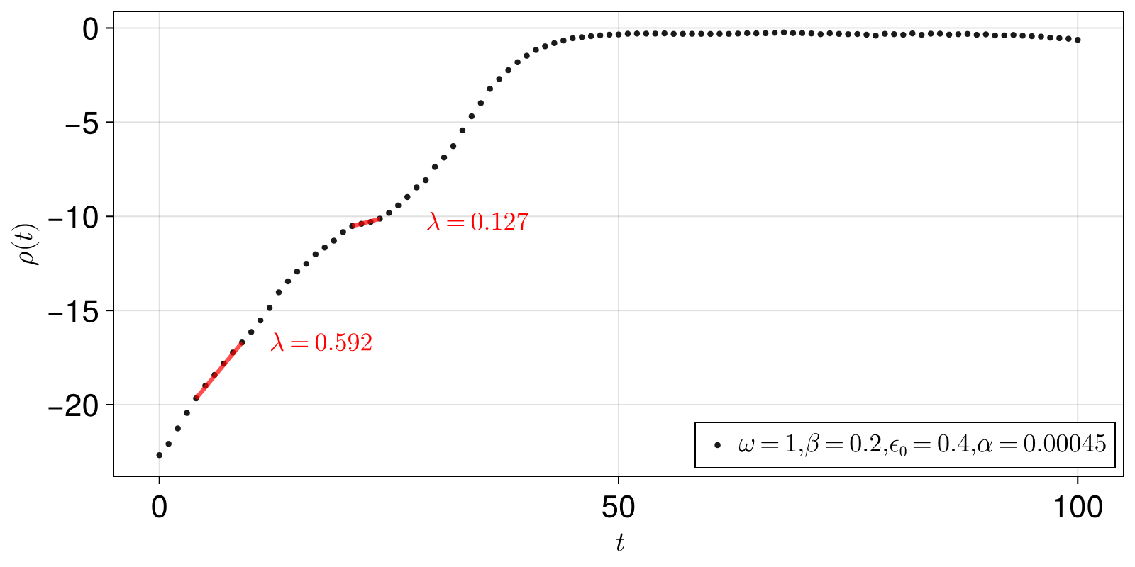
- Lyapunov1992A. M. Lyapunov, The General Problem of the Stability of Motion, Taylor & Francis (1992)
- Geist1990K. Geist et al., Progr. Theor. Phys. 83, pp 875 (1990)
- Benettin1980G. Benettin et al., Meccanica 15, pp 9-20 & 21-30 (1980)
- DatserisParlitz2022Datseris & Parlitz 2022, Nonlinear Dynamics: A Concise Introduction Interlaced with Code, Springer Nature, Undergrad. Lect. Notes In Physics
- Benettin1976G. Benettin et al., Phys. Rev. A 14, pp 2338 (1976)
- Skokos2016Skokos, C. H. et al., Chaos Detection and Predictability - Chapter 1 (section 1.3.2), Lecture Notes in Physics 915, Springer (2016)
- Kantz1994Kantz, H., Phys. Lett. A 185, pp 77–87 (1994)
- JánosiTél2024Dániel Jánosi, Tamás Tél, Phys. Rep. 1092, pp 1-64 (2024)