Examples

In this page we go through various examples of combining processes to make models that have been already used in the literature, or using DynamicalSystems.jl or other packages to analyse conceptual climate models.

Classic Snowball Earth hysteresis

The origins of energy balance models ((Sellers, 1969; Budyko, 1969; Ghil, 1981; North et al., 1981)) examined the impact of variations in insolation on the global climate. In particular, they studied how simple energy balance models with only ice-albedo and water vapor feedbacks yielded bi-stable hysteresis between a cold "snowball" state and a warm Earth, as the solar constant was varied. The same kind of behaviour is also used in (Datseris and Parlitz, 2022; Ch. 2) as an introductory example to dynamical systems.

We can easily replicate such a model by creating a global-mean temperature model without even having the water vapor feedback. We will combine the processes:

using ConceptualClimateModels
using ConceptualClimateModels.CCMV

budyko_processes = [
    BasicRadiationBalance(),
    EmissivityStefanBoltzmanOLR(),
    IceAlbedoFeedback(; min = 0.3, max = 0.7),
    α ~ α_ice,
    ParameterProcess(ε), # emissivity is a parameter
    f ~ 0, # no external forcing
    # absorbed solar radiation has a default process
]

budyko = processes_to_coupledodes(budyko_processes)
println(dynamical_system_summary(budyko))

1-dimensional CoupledODEs
 deterministic: true
 discrete time: false
 in-place:      false

with equations:
 Differential(t)(T(t)) ~ (-0.0029390154298310064(ASR(t) + f(t) - OLR(t))) / (-τ_T)
 ε(t) ~ ε_0
 f(t) ~ 0.0
 S(t) ~ 1.0
 α_ice(t) ~ max_α_ice + 0.5(-max_α_ice + min_α_ice)*(1 + tanh((2(-Tfreeze_α_ice + (1//2)*Tscale_α_ice + T(t))) / Tscale_α_ice))
 OLR(t) ~ 5.670374419e-8ε(t)*(T(t)^4)
 α(t) ~ α_ice(t)
 ASR(t) ~ 340.25S(t)*(1 - α(t))

and parameter values:
 τ_T ~ 1.4695077149155033e6
 Tfreeze_α_ice ~ 273.15
 min_α_ice ~ 0.3
 max_α_ice ~ 0.7
 Tscale_α_ice ~ 10.0
 ε_0 ~ 0.5

We can perform a typical hysteresis loop analysis straightforwardly by doing a continuation analysis with the Attractors.jl subpackage of DynamicalSystems.jl.

For setting up the continuation we leverage the integration with DynamicalSystems.jl:

using DynamicalSystems

grid = physically_plausible_grid(budyko)
mapper = AttractorsViaRecurrences(budyko, grid)
rfam = RecurrencesFindAndMatch(mapper)
sampler = physically_plausible_ic_sampler(budyko)
sampler() # randomly sample initial conditions

1-element Vector{Float64}:
 295.57915724019756

Now, to obtain the symbolic parameter index corresponding to the insolation parameter, there are several ways as described in the main tutorial. The simplest way is

index = :ε_0

:ε_0

Now we perform the continuation versus the effective emissivity, to approximate increasing or decreasing the strength of the greenhouse effect:

εrange = 0.3:0.01:0.8
fractions_curves, attractors_info = continuation(
    rfam, εrange, index, sampler;
    samples_per_parameter = 1000,
    show_progress = false,
)

([Dict(1 => 1.0), Dict(1 => 1.0), Dict(1 => 1.0), Dict(1 => 1.0), Dict(1 => 1.0), Dict(1 => 1.0), Dict(1 => 1.0), Dict(1 => 1.0), Dict(1 => 1.0), Dict(1 => 1.0)  …  Dict(2 => 1.0), Dict(2 => 1.0), Dict(2 => 1.0), Dict(2 => 1.0), Dict(2 => 1.0), Dict(2 => 1.0), Dict(2 => 1.0), Dict(2 => 1.0), Dict(2 => 1.0), Dict(2 => 1.0)], Dict{Int64, StateSpaceSet{1, Float64}}[Dict(1 => 1-dimensional StateSpaceSet{Float64} with 1 points), Dict(1 => 1-dimensional StateSpaceSet{Float64} with 1 points), Dict(1 => 1-dimensional StateSpaceSet{Float64} with 1 points), Dict(1 => 1-dimensional StateSpaceSet{Float64} with 1 points), Dict(1 => 1-dimensional StateSpaceSet{Float64} with 1 points), Dict(1 => 1-dimensional StateSpaceSet{Float64} with 1 points), Dict(1 => 1-dimensional StateSpaceSet{Float64} with 1 points), Dict(1 => 1-dimensional StateSpaceSet{Float64} with 1 points), Dict(1 => 1-dimensional StateSpaceSet{Float64} with 1 points), Dict(1 => 1-dimensional StateSpaceSet{Float64} with 1 points)  …  Dict(2 => 1-dimensional StateSpaceSet{Float64} with 1 points), Dict(2 => 1-dimensional StateSpaceSet{Float64} with 1 points), Dict(2 => 1-dimensional StateSpaceSet{Float64} with 1 points), Dict(2 => 1-dimensional StateSpaceSet{Float64} with 1 points), Dict(2 => 1-dimensional StateSpaceSet{Float64} with 1 points), Dict(2 => 1-dimensional StateSpaceSet{Float64} with 1 points), Dict(2 => 1-dimensional StateSpaceSet{Float64} with 1 points), Dict(2 => 1-dimensional StateSpaceSet{Float64} with 1 points), Dict(2 => 1-dimensional StateSpaceSet{Float64} with 1 points), Dict(2 => 1-dimensional StateSpaceSet{Float64} with 1 points)])

and visualize it

using CairoMakie
a2r = A -> first(first(A)) # plot attractor: extract first point and first dimension of point
plot_basins_attractors_curves(fractions_curves, attractors_info, a2r, εrange)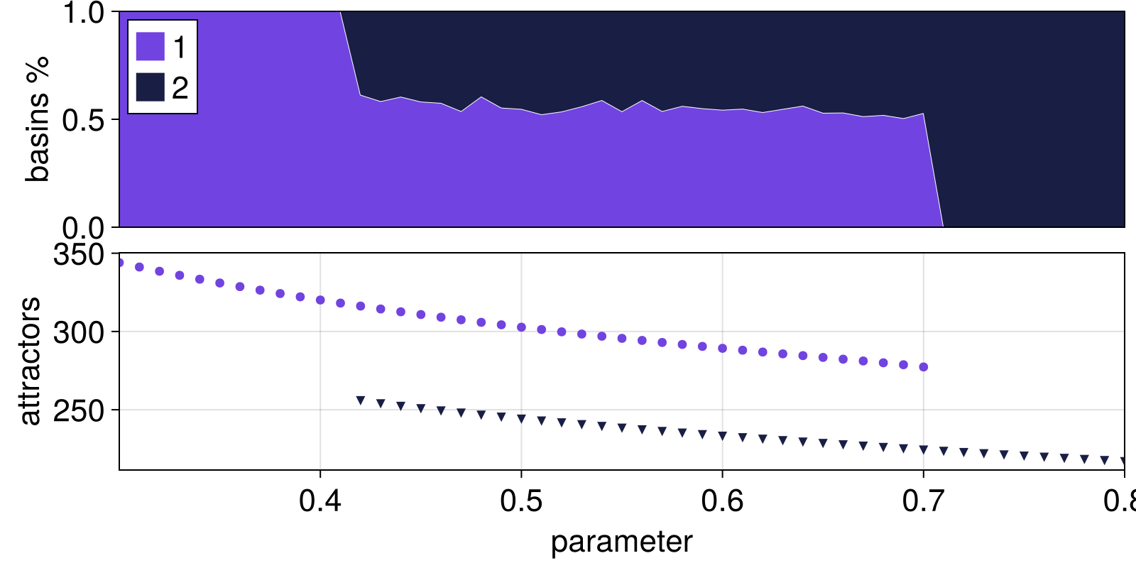

we see there are two attractors at low and high temperatures and that they have approximately the same basin fractions of 50% each.

Rate dependent tipping in the Stommel model

The Stommel model is a good example for rate dependent tipping (Lohmann et al., 2021). We can modify the process ΔTStommelModel and make its parameter η3 be a time- dependent variable instead, like so:

using ConceptualClimateModels
using ConceptualClimateModels.CCMV

@variables η1(t)
@parameters η1_0 = 2.0 # starting value for η1 parameter
@parameters r_η = 0.0  # the rate that η1 changes

processes = [
    ΔTStommelModel(; η1 = η1), # replace keyword with a symbolic variable
    η1 ~ η1_0 + r_η*t, # this symbolic variable has its own equation!
]

stommel = processes_to_coupledodes(processes)
println(dynamical_system_summary(stommel))

2-dimensional CoupledODEs
 deterministic: true
 discrete time: false
 in-place:      false

with equations:
 Differential(t)(ΔT(t)) ~ η1(t) - ΔT(t) - ΔT(t)*abs(-ΔS(t) + ΔT(t))
 Differential(t)(ΔS(t)) ~ η2 - ΔS(t)*abs(-ΔS(t) + ΔT(t)) - ΔS(t)*η3
 η1(t) ~ η1_0 + r_η*t

and parameter values:
 r_η ~ 0.0
 η1_0 ~ 2.0
 η2 ~ 1.0
 η3 ~ 0.3

At the moment r_η = 0 and the system is autonomous. Hence, we can easily estimate its bifurcation diagram using the same steps as the above example.

using DynamicalSystems

grid = physically_plausible_grid(stommel)
mapper = AttractorsViaRecurrences(stommel, grid;
    consecutive_recurrences = 1000, attractor_locate_steps = 10,
)
rfam = RecurrencesFindAndMatch(mapper)
sampler = physically_plausible_ic_sampler(stommel)

ηrange = 2.0:0.01:4.0
fractions_curves, attractors_info = continuation(
    rfam, ηrange, η1_0, sampler;
    samples_per_parameter = 1000,
    show_progress = false,
)

([Dict(1 => 1.0), Dict(1 => 1.0), Dict(1 => 1.0), Dict(1 => 1.0), Dict(1 => 1.0), Dict(1 => 1.0), Dict(1 => 1.0), Dict(1 => 1.0), Dict(1 => 1.0), Dict(1 => 1.0)  …  Dict(2 => 1.0), Dict(2 => 1.0), Dict(2 => 1.0), Dict(2 => 1.0), Dict(2 => 1.0), Dict(2 => 1.0), Dict(2 => 1.0), Dict(2 => 1.0), Dict(2 => 1.0), Dict(2 => 1.0)], Dict{Int64, StateSpaceSet{2, Float64}}[Dict(1 => 2-dimensional StateSpaceSet{Float64} with 1 points), Dict(1 => 2-dimensional StateSpaceSet{Float64} with 1 points), Dict(1 => 2-dimensional StateSpaceSet{Float64} with 1 points), Dict(1 => 2-dimensional StateSpaceSet{Float64} with 1 points), Dict(1 => 2-dimensional StateSpaceSet{Float64} with 1 points), Dict(1 => 2-dimensional StateSpaceSet{Float64} with 1 points), Dict(1 => 2-dimensional StateSpaceSet{Float64} with 1 points), Dict(1 => 2-dimensional StateSpaceSet{Float64} with 1 points), Dict(1 => 2-dimensional StateSpaceSet{Float64} with 1 points), Dict(1 => 2-dimensional StateSpaceSet{Float64} with 1 points)  …  Dict(2 => 2-dimensional StateSpaceSet{Float64} with 1 points), Dict(2 => 2-dimensional StateSpaceSet{Float64} with 1 points), Dict(2 => 2-dimensional StateSpaceSet{Float64} with 1 points), Dict(2 => 2-dimensional StateSpaceSet{Float64} with 1 points), Dict(2 => 2-dimensional StateSpaceSet{Float64} with 1 points), Dict(2 => 2-dimensional StateSpaceSet{Float64} with 1 points), Dict(2 => 2-dimensional StateSpaceSet{Float64} with 1 points), Dict(2 => 2-dimensional StateSpaceSet{Float64} with 1 points), Dict(2 => 2-dimensional StateSpaceSet{Float64} with 1 points), Dict(2 => 2-dimensional StateSpaceSet{Float64} with 1 points)])

and visualize it

using CairoMakie
a2r = A -> first(first(A)) # plot attractor: extract first point and first dimension of point
fig = plot_attractors_curves(attractors_info, a2r, ηrange)
ax = content(fig[1,1])
ax.ylabel = "ΔT - fixed points"
ax.xlabel = "parameter η1"
fig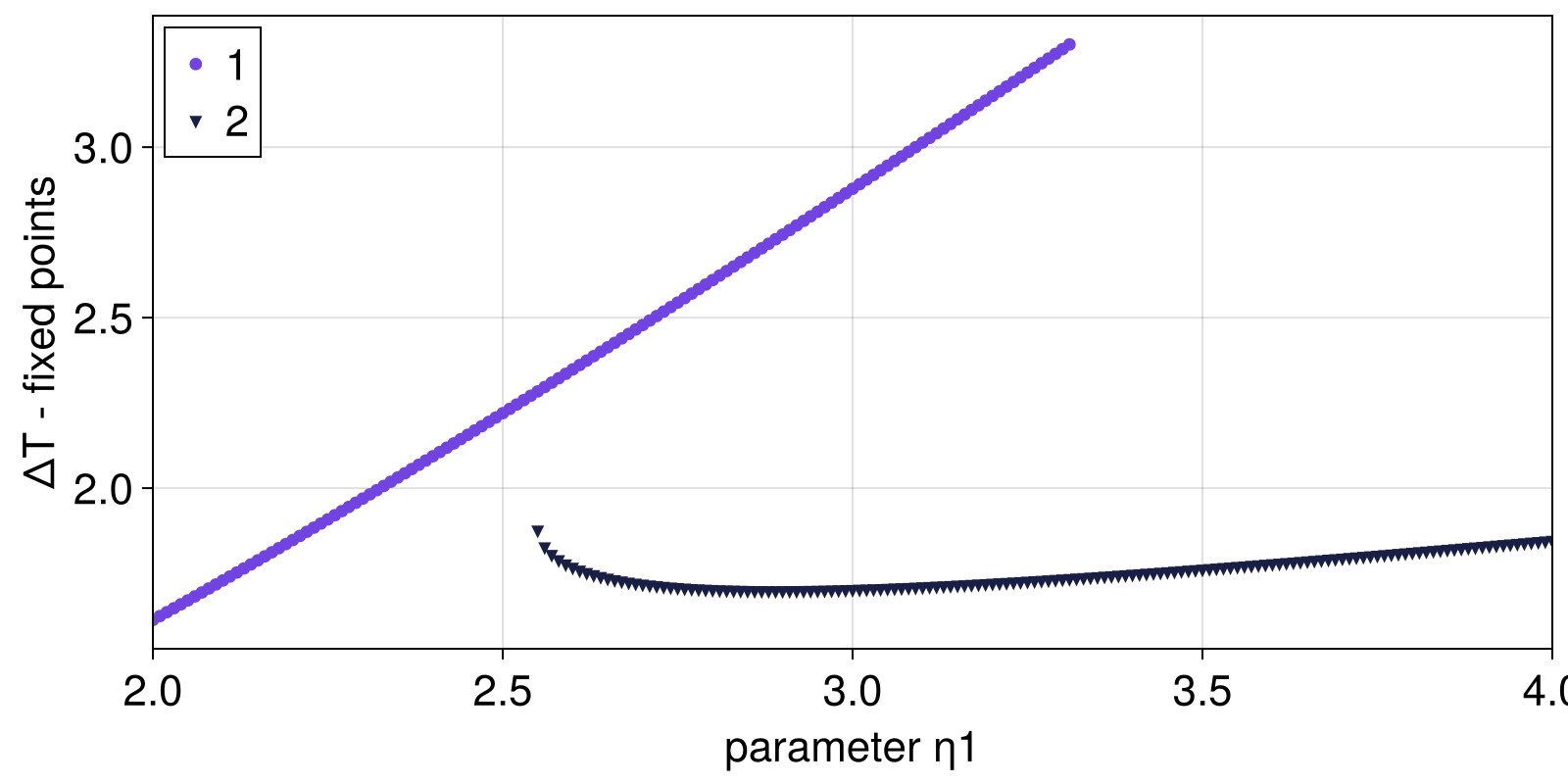

Alright, now we can perform simple simulations where we evolve the system forwards in time while η_1 increases at different rates. We can use the trajectory function to evolve it and due to the nice integration between DynamicalSystems.jl and ModelingToolkit.jl we can use any "observable" of the system for the trajectory output.

r1, r2 = 0.02, 0.2
u0 = [1.61334  1.85301] # always start from same state
set_parameter!(stommel, η1_0, 2.0) # set it to initial value

for (j, r) in enumerate((r1, r2))
    # update the named parameter `r_η` to the numeric value `r`
    set_parameter!(stommel, r_η, r)
    # simulate until η1 becomes 4
    tfinal = (4.0 - default_value(η1_0))/r
    # trajectory: first column = ΔΤ, second column = η1
    X, tvec = trajectory(stommel, tfinal, u0; save_idxs = [ΔT, η1])
    lines!(ax, X[:, 2], X[:, 1]; color = Cycled(j+2), label = "r_η = $(r)")
end
axislegend(ax; unique = true, position = :lt)
ylims!(ax, 1, 4)
fig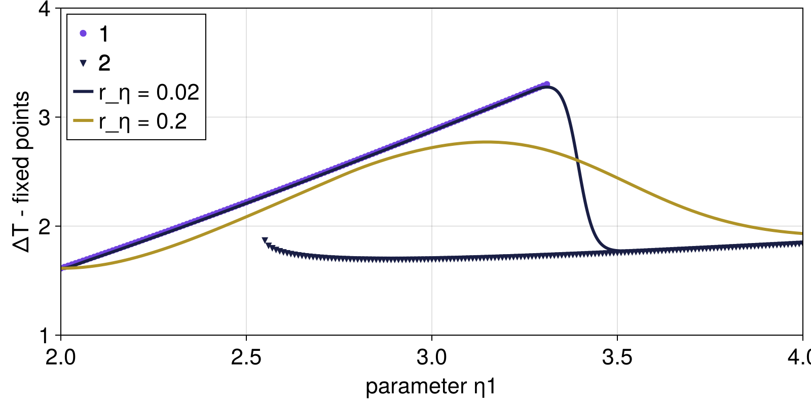

As you can see from the figure, depending on the rate the system either "tracks" the fixed point of high ΔΤ or it collapses down to the small ΔT branch. This happens because the system crosses the unstable manifold of the lower branch (Datseris and Parlitz, 2022; Chap. 12). To visualize the unstable manifold we could use BifurcationKit.jl, however, it is very inconvenient to do so, because BifurcationKit.jl does not provide most of the conveniences that DynamicalSystems.jl does. For example, it does not integrate well enough with DifferentialEquations.jl (to allow passing ODEProblem which is created by DynamicalSystem). It also does not allow indexing parameters by their symbolic bindings. Lastly, it does not work with models generated with ModelingToolkit.jl so we would have to re-write all the equations that the chosen processes made for us.

Glacial oscillations

Coming soon!