CloudToppedMixedLayerModel

using DynamicalSystems, ConceptualClimateModels
import ConceptualClimateModels.CloudToppedMixedLayerModel as CTMLM

Precompiling DynamicalSystems...
   1853.8 ms  ? DiffEqBase
   1247.1 ms  ? DiffEqBase → DiffEqBaseChainRulesCoreExt
   1315.9 ms  ? DiffEqBase → DiffEqBaseForwardDiffExt
   1430.0 ms  ? DiffEqBase → DiffEqBaseMeasurementsExt
   1505.3 ms  ? DiffEqBase → DiffEqBaseSparseArraysExt
   1843.9 ms  ? DiffEqBase → DiffEqBaseDistributionsExt
   1176.9 ms  ? OrdinaryDiffEqCore
    666.8 ms  ? OrdinaryDiffEqCore → OrdinaryDiffEqCoreEnzymeCoreExt
    665.7 ms  ? OrdinaryDiffEqTsit5
   1589.7 ms  ? DynamicalSystemsBase
   1129.6 ms  ? Attractors
   1210.3 ms  ? ChaosTools
   1214.1 ms  ? PredefinedDynamicalSystems
Info Given DynamicalSystems was explicitly requested, output will be shown live 
┌ Warning: Module DynamicalSystemsBase with build ID ffffffff-ffff-ffff-2932-4fe4f54132dc is missing from the cache.
│ This may mean DynamicalSystemsBase [6e36e845-645a-534a-86f2-f5d4aa5a06b4] does not support precompilation but is imported by a module that does.
└ @ Base loading.jl:2541
   1095.1 ms  ? DynamicalSystems
┌ Warning: Module DynamicalSystemsBase with build ID ffffffff-ffff-ffff-2932-4fe4f54132dc is missing from the cache.
│ This may mean DynamicalSystemsBase [6e36e845-645a-534a-86f2-f5d4aa5a06b4] does not support precompilation but is imported by a module that does.
└ @ Base loading.jl:2541
Precompiling DiffEqBaseMeasurementsExt...
   1791.8 ms  ? DiffEqBase
Info Given DiffEqBaseMeasurementsExt was explicitly requested, output will be shown live 
┌ Warning: Module DiffEqBase with build ID ffffffff-ffff-ffff-0382-96b11dc327db is missing from the cache.
│ This may mean DiffEqBase [2b5f629d-d688-5b77-993f-72d75c75574e] does not support precompilation but is imported by a module that does.
└ @ Base loading.jl:2541
    704.2 ms  ? DiffEqBase → DiffEqBaseMeasurementsExt
┌ Warning: Module DiffEqBase with build ID ffffffff-ffff-ffff-0382-96b11dc327db is missing from the cache.
│ This may mean DiffEqBase [2b5f629d-d688-5b77-993f-72d75c75574e] does not support precompilation but is imported by a module that does.
└ @ Base loading.jl:2541
Precompiling PredefinedDynamicalSystems...
   1778.9 ms  ? DiffEqBase
   1067.4 ms  ? DiffEqBase → DiffEqBaseForwardDiffExt
   1122.8 ms  ? OrdinaryDiffEqCore
   1262.6 ms  ? DiffEqBase → DiffEqBaseSparseArraysExt
    685.5 ms  ? OrdinaryDiffEqCore → OrdinaryDiffEqCoreEnzymeCoreExt
    658.8 ms  ? OrdinaryDiffEqTsit5
   1586.5 ms  ? DynamicalSystemsBase
Info Given PredefinedDynamicalSystems was explicitly requested, output will be shown live 
┌ Warning: Module DynamicalSystemsBase with build ID ffffffff-ffff-ffff-2932-4fe4f54132dc is missing from the cache.
│ This may mean DynamicalSystemsBase [6e36e845-645a-534a-86f2-f5d4aa5a06b4] does not support precompilation but is imported by a module that does.
└ @ Base loading.jl:2541
    792.5 ms  ? PredefinedDynamicalSystems
┌ Warning: Module DynamicalSystemsBase with build ID ffffffff-ffff-ffff-2932-4fe4f54132dc is missing from the cache.
│ This may mean DynamicalSystemsBase [6e36e845-645a-534a-86f2-f5d4aa5a06b4] does not support precompilation but is imported by a module that does.
└ @ Base loading.jl:2541
Precompiling Attractors...
   1799.9 ms  ? DiffEqBase
   1061.3 ms  ? DiffEqBase → DiffEqBaseForwardDiffExt
   1301.6 ms  ? DiffEqBase → DiffEqBaseSparseArraysExt
   1528.6 ms  ? DiffEqBase → DiffEqBaseDistributionsExt
   1593.0 ms  ? OrdinaryDiffEqCore
    694.9 ms  ? OrdinaryDiffEqCore → OrdinaryDiffEqCoreEnzymeCoreExt
    678.0 ms  ? OrdinaryDiffEqTsit5
   1573.9 ms  ? DynamicalSystemsBase
Info Given Attractors was explicitly requested, output will be shown live 
┌ Warning: Module DynamicalSystemsBase with build ID ffffffff-ffff-ffff-2932-4fe4f54132dc is missing from the cache.
│ This may mean DynamicalSystemsBase [6e36e845-645a-534a-86f2-f5d4aa5a06b4] does not support precompilation but is imported by a module that does.
└ @ Base loading.jl:2541
   1130.6 ms  ? Attractors
┌ Warning: Module DynamicalSystemsBase with build ID ffffffff-ffff-ffff-2932-4fe4f54132dc is missing from the cache.
│ This may mean DynamicalSystemsBase [6e36e845-645a-534a-86f2-f5d4aa5a06b4] does not support precompilation but is imported by a module that does.
└ @ Base loading.jl:2541
Precompiling AttractorsVisualizations...
   1774.7 ms  ? DiffEqBase
   1230.0 ms  ? DiffEqBase → DiffEqBaseForwardDiffExt
   1292.9 ms  ? DiffEqBase → DiffEqBaseUnitfulExt
   1335.7 ms  ? DiffEqBase → DiffEqBaseChainRulesCoreExt
   1531.9 ms  ? DiffEqBase → DiffEqBaseSparseArraysExt
   1796.5 ms  ? DiffEqBase → DiffEqBaseDistributionsExt
   1212.9 ms  ? OrdinaryDiffEqCore
    683.7 ms  ? OrdinaryDiffEqCore → OrdinaryDiffEqCoreEnzymeCoreExt
    677.7 ms  ? OrdinaryDiffEqTsit5
   1566.5 ms  ? DynamicalSystemsBase
   1103.6 ms  ? Attractors
Info Given AttractorsVisualizations was explicitly requested, output will be shown live 
┌ Warning: Module Attractors with build ID ffffffff-ffff-ffff-4a1b-fd491f3f4bfc is missing from the cache.
│ This may mean Attractors [f3fd9213-ca85-4dba-9dfd-7fc91308fec7] does not support precompilation but is imported by a module that does.
└ @ Base loading.jl:2541
    698.4 ms  ? Attractors → AttractorsVisualizations
┌ Warning: Module Attractors with build ID ffffffff-ffff-ffff-4a1b-fd491f3f4bfc is missing from the cache.
│ This may mean Attractors [f3fd9213-ca85-4dba-9dfd-7fc91308fec7] does not support precompilation but is imported by a module that does.
└ @ Base loading.jl:2541
Precompiling ChaosTools...
   1814.8 ms  ? DiffEqBase
   1200.1 ms  ? DiffEqBase → DiffEqBaseMeasurementsExt
   1268.6 ms  ? DiffEqBase → DiffEqBaseForwardDiffExt
   1557.8 ms  ? DiffEqBase → DiffEqBaseSparseArraysExt
   1805.1 ms  ? DiffEqBase → DiffEqBaseDistributionsExt
   1814.1 ms  ? OrdinaryDiffEqCore
    689.1 ms  ? OrdinaryDiffEqCore → OrdinaryDiffEqCoreEnzymeCoreExt
    680.4 ms  ? OrdinaryDiffEqTsit5
   1574.7 ms  ? DynamicalSystemsBase
Info Given ChaosTools was explicitly requested, output will be shown live 
┌ Warning: Module DynamicalSystemsBase with build ID ffffffff-ffff-ffff-2932-4fe4f54132dc is missing from the cache.
│ This may mean DynamicalSystemsBase [6e36e845-645a-534a-86f2-f5d4aa5a06b4] does not support precompilation but is imported by a module that does.
└ @ Base loading.jl:2541
    787.1 ms  ? ChaosTools
┌ Warning: Module DynamicalSystemsBase with build ID ffffffff-ffff-ffff-2932-4fe4f54132dc is missing from the cache.
│ This may mean DynamicalSystemsBase [6e36e845-645a-534a-86f2-f5d4aa5a06b4] does not support precompilation but is imported by a module that does.
└ @ Base loading.jl:2541
Precompiling DynamicalSystemsVisualizations...
   1783.6 ms  ? DiffEqBase
   1212.4 ms  ? DiffEqBase → DiffEqBaseForwardDiffExt
   1315.9 ms  ? DiffEqBase → DiffEqBaseMeasurementsExt
   1367.1 ms  ? DiffEqBase → DiffEqBaseChainRulesCoreExt
   1482.4 ms  ? DiffEqBase → DiffEqBaseSparseArraysExt
   2121.9 ms  ? DiffEqBase → DiffEqBaseDistributionsExt
   1024.5 ms  ? DiffEqBase → DiffEqBaseUnitfulExt
   1186.1 ms  ? OrdinaryDiffEqCore
    685.4 ms  ? OrdinaryDiffEqCore → OrdinaryDiffEqCoreEnzymeCoreExt
    688.1 ms  ? OrdinaryDiffEqTsit5
   1584.2 ms  ? DynamicalSystemsBase
    788.5 ms  ? ChaosTools
   1059.7 ms  ? PredefinedDynamicalSystems
   1403.4 ms  ? Attractors
    689.8 ms  ? Attractors → AttractorsVisualizations
   1122.5 ms  ? DynamicalSystems
Info Given DynamicalSystemsVisualizations was explicitly requested, output will be shown live 
┌ Warning: Module DynamicalSystems with build ID ffffffff-ffff-ffff-823e-45682b8f527f is missing from the cache.
│ This may mean DynamicalSystems [61744808-ddfa-5f27-97ff-6e42cc95d634] does not support precompilation but is imported by a module that does.
└ @ Base loading.jl:2541
    677.8 ms  ? DynamicalSystems → DynamicalSystemsVisualizations
┌ Warning: Module DynamicalSystems with build ID ffffffff-ffff-ffff-823e-45682b8f527f is missing from the cache.
│ This may mean DynamicalSystems [61744808-ddfa-5f27-97ff-6e42cc95d634] does not support precompilation but is imported by a module that does.
└ @ Base loading.jl:2541

Fixed states of Stevens 2006

Here we want to recreate the same bulk boundary layer model defined in (Stevens, 2006), equations 31-33.

const cₚ = 1004.0 # heat capacity at constant pressure (J/K/kg)

eqs = [
    CTMLM.mlm_dynamic(),
    CTMLM.entrainment_velocity(:Stevens2006; use_augmentation = false),
    ## Figure 1 and Sec. 4.2 provide these values:
    CTMLM.s₊ ~ 301200.0/cₚ,
    CTMLM.q₊ ~ 1.56,
    CTMLM.s₀ ~ CTMLM.s₊ - 12.5,
    CTMLM.ρ₀ ~ 1,
    CTMLM.q₀ ~ CTMLM.q_saturation(288.96 + 1.25),
    CTMLM.ΔF_s ~ 40.0
]

8-element Vector{Any}:
 TimeDerivative[TimeDerivative(z_b(t), -w_m(t) + w_e(t) - D*z_b(t), LiteralParameter{Float64}(1.1574074074074073e-5)), TimeDerivative(s_b(t), -1.1574074074074073e-5s_x(t) + ((0.00099601593625498(SHF(t) - ΔF_s(t))) / ρ₀(t) + Δ₊s(t)*w_e(t)) / z_b(t), LiteralParameter{Float64}(1.1574074074074073e-5)), TimeDerivative(q_b(t), -1.1574074074074073e-5q_x(t) + ((-ΔF_q(t) + LHF(t)) / (2530.0ρ₀(t)) + Δ₊q(t)*w_e(t)) / z_b(t), LiteralParameter{Float64}(1.1574074074074073e-5))]
 w_e(t) ~ (e_e*ΔF_s(t)) / (1004.0Δ₊s(t)*ρ₀(t))
 s₊(t) ~ 300.0
 q₊(t) ~ 1.56
 s₀(t) ~ -12.5 + s₊(t)
 ρ₀(t) ~ 1
 q₀(t) ~ 12.404970818808321
 ΔF_s(t) ~ 40.0

We now give these equations to the main function that creates a DynamicalSystem from the processes (and we also provide CTMLM to obtain default processes from)

ds = processes_to_coupledodes(eqs, CTMLM)

3-dimensional CoupledODEs
 deterministic: true
 discrete time: false
 in-place:      false
 dynamic rule:  GeneratedFunctionWrapper
 ODE solver:    Tsit5
 ODE kwargs:    (abstol = 1.0e-6, reltol = 1.0e-6)
 parameters:    [0.9, 3.0e-6, 0.0012, 6.0, 0.0, 0.0, 0.0, 0.0, 0.0, 0.0  …  0.0, 0.0, 0.0, 0.0, 0.0, 0.0, 0.0, 0.0, 0.0, 0.0]
 time:          0.0
 state:         [11.0, 290.0, 1200.0]

We also make sure to use the same parameter values as in the paper:

set_parameter!(ds, :D, 4e-6)
set_parameter!(ds, :d_c, 0.0011)
set_parameter!(ds, :U, 0.008/0.0011) # U*d_c = 0.008
set_parameter!(ds, :e_e, 1.0) # effective emissivity

And that's all. We can run the system to its steady state:

step!(ds, 100.0)

3-dimensional CoupledODEs
 deterministic: true
 discrete time: false
 in-place:      false
 dynamic rule:  GeneratedFunctionWrapper
 ODE solver:    Tsit5
 ODE kwargs:    (abstol = 1.0e-6, reltol = 1.0e-6)
 parameters:    [1.0, 4.0e-6, 0.0011, 7.2727272727272725, 0.0, 0.0, 0.0, 0.0, 0.0, 0.0  …  0.0, 0.0, 0.0, 0.0, 0.0, 0.0, 0.0, 0.0, 0.0, 0.0]
 time:          100.10196159861358
 state:         [9.315240208837562, 287.4999999999997, 796.8127490039915]

leading to a steady state with height $z_b$ ($h_\infty$ in (Stevens, 2006)) of about 800 meters as in the paper. Extracting the variable $\sigma$ of Eq. 38 is also very easy:

Δs = CTMLM.s₊ - CTMLM.s₀ # symbolic variable not existing in the graph of the `ds`
σ = observe_state(ds, CTMLM.V * Δs / CTMLM.ΔF_s * cₚ)

2.5100000000000002

and we get the same value (note multiplication by cₚ, because s is in units of K).

If you want to see a list of all equations that compose the dynamical system then do

all_equations(ds)

\[ \begin{align} \frac{\mathrm{d} \mathtt{q\_b}\left( t \right)}{\mathrm{d}t} &= - 86400 \left( 1.1574 \cdot 10^{-5} \mathtt{q\_x}\left( t \right) + \frac{\frac{\mathtt{{\Delta}F\_q}\left( t \right) - \mathtt{LHF}\left( t \right)}{2530 \mathtt{\rho_0}\left( t \right)} - \mathtt{\Delta.q}\left( t \right) \mathtt{w\_e}\left( t \right)}{\mathtt{z\_b}\left( t \right)} \right) \\ \frac{\mathrm{d} \mathtt{s\_b}\left( t \right)}{\mathrm{d}t} &= - 86400 \left( \frac{\frac{ - 0.00099602 \left( \mathtt{SHF}\left( t \right) - \mathtt{{\Delta}F\_s}\left( t \right) \right)}{\mathtt{\rho_0}\left( t \right)} - \mathtt{\Delta.s}\left( t \right) \mathtt{w\_e}\left( t \right)}{\mathtt{z\_b}\left( t \right)} + 1.1574 \cdot 10^{-5} \mathtt{s\_x}\left( t \right) \right) \\ \frac{\mathrm{d} \mathtt{z\_b}\left( t \right)}{\mathrm{d}t} &= - 86400 \left( \mathtt{w\_m}\left( t \right) - \mathtt{w\_e}\left( t \right) + D \mathtt{z\_b}\left( t \right) \right) \\ \mathtt{\rho_0}\left( t \right) &= 1 \\ \mathtt{s.}\left( t \right) &= 300 \\ \mathtt{{\Delta}F\_s}\left( t \right) &= 40 \\ \mathtt{q_0}\left( t \right) &= 12.405 \\ V\left( t \right) &= U \mathtt{d\_c} \\ \mathtt{q\_x}\left( t \right) &= 0 \\ \mathtt{s\_x}\left( t \right) &= 0 \\ \mathtt{w\_m}\left( t \right) &= 0 \\ \mathtt{{\Delta}F\_q}\left( t \right) &= 0 \\ \mathtt{q.}\left( t \right) &= 1.56 \\ \mathtt{\Delta.s}\left( t \right) &= - \mathtt{s\_b}\left( t \right) + \mathtt{s.}\left( t \right) \\ \mathtt{s_0}\left( t \right) &= -12.5 + \mathtt{s.}\left( t \right) \\ \mathtt{\Delta_{0}q}\left( t \right) &= \mathtt{q\_b}\left( t \right) - \mathtt{q_0}\left( t \right) \\ \mathtt{\Delta.q}\left( t \right) &= - \mathtt{q\_b}\left( t \right) + \mathtt{q.}\left( t \right) \\ \mathtt{w\_e}\left( t \right) &= \frac{\mathtt{e\_e} \mathtt{{\Delta}F\_s}\left( t \right)}{1004 \mathtt{\Delta.s}\left( t \right) \mathtt{\rho_0}\left( t \right)} \\ \mathtt{\Delta_{0}s}\left( t \right) &= \mathtt{s\_b}\left( t \right) - \mathtt{s_0}\left( t \right) \\ \mathtt{LHF}\left( t \right) &= - 2530 \mathtt{\Delta_{0}q}\left( t \right) V\left( t \right) \mathtt{\rho_0}\left( t \right) \\ \mathtt{SHF}\left( t \right) &= - 1004 V\left( t \right) \mathtt{\rho_0}\left( t \right) \mathtt{\Delta_{0}s}\left( t \right) \end{align} \]

In the compiled documentation these render via LaTeX but running this in the REPL won't be as pretty :)

Adding clouds

We can add clouds to the mixed layer model using the same decoupling-based approach as in (Datseris, 2025) (while keeping SST a fixed boundary condition) just by including a couple more equations to the ones already defined, so that $C, \mathcal{D}$ have a process assigned to them. We will also augment ΔF to be partially proportional to C using a very simple ad-hoc approach.

eqs = [
    CTMLM.mlm_dynamic(),
    CTMLM.entrainment_velocity(:Stevens2006; use_augmentation = false),
    ## Cloud stuff
    CTMLM.cf_dynamic(),
    CTMLM.decoupling_variable(),
    CTMLM.cloud_base_height(:Bolton1980),
    CTMLM.CTRC ~ 10 + 40*CTMLM.C, # cloud top radiative cooling
    CTMLM.ΔF_s ~ CTMLM.CTRC, # same equation
    ## rest the same
    CTMLM.s₊ ~ 301200.0/cₚ,
    CTMLM.q₊ ~ 1.56,
    CTMLM.s₀ ~ CTMLM.s₊ - 12.5,
    CTMLM.ρ₀ ~ 1,
    CTMLM.q₀ ~ CTMLM.q_saturation(288.96 + 1.25),
]

ds = processes_to_coupledodes(eqs, CTMLM)

4-dimensional CoupledODEs
 deterministic: true
 discrete time: false
 in-place:      false
 dynamic rule:  GeneratedFunctionWrapper
 ODE solver:    Tsit5
 ODE kwargs:    (abstol = 1.0e-6, reltol = 1.0e-6)
 parameters:    [0.9, 3.0e-6, 1.0, 0.2, 1.0, 0.5, 100.0, 2.0, 0.0012, 6.0  …  0.0, 0.0, 0.0, 0.0, 0.0, 0.0, 0.0, 0.0, 0.0, 0.0]
 time:          0.0
 state:         [11.0, 290.0, 1200.0, 1.0]

And we run the model to a steady state:

set_parameter!(ds, :D, 4e-6)
set_parameter!(ds, :d_c, 0.0009)
set_parameter!(ds, :U, 6.8) # U*d_c = 0.008
set_parameter!(ds, :e_e, 1.0) # effective emissivity

step!(ds, 100.0)
observe_state.(ds, (:z_b, :q_b, :s_b, :C)) # get state variables by name

(763.5014057710669, 8.794700233030296, 287.50000000000017, 0.7081938746297317)

Climate change scenario: increasing SST

If you want to study multistability for alternate cloud states (Cumulus vs Stratocumulus), or perform continuations (like the climate change scenarios in (Datseris, 2025)), visit the documentation of Attractors.jl.

As a brief example we will perform a simple climate change scenario where SST increases with a constant rate. First, we modify the equations so that s₀, q₀ are derived from a prescribed SST:

@parameters SST = 290.0
eqs = [
    CTMLM.mlm_dynamic(),
    CTMLM.entrainment_velocity(:Stevens2006; use_augmentation = false),
    ## Cloud stuff
    CTMLM.cf_dynamic(),
    CTMLM.decoupling_variable(),
    CTMLM.cloud_base_height(:Bolton1980),
    CTMLM.CTRC ~ 10 + 40*CTMLM.C, # cloud top radiative cooling
    CTMLM.ΔF_s ~ CTMLM.CTRC, # same equation
    ## Usage of SST
    CTMLM.s₀ ~ SST,
    CTMLM.q₀ ~ CTMLM.q_saturation(SST),
    ## rest the same
    CTMLM.s₊ ~ 301200.0/cₚ,
    CTMLM.q₊ ~ 1.56,
    CTMLM.ρ₀ ~ 1,
]

ds = processes_to_coupledodes(eqs, CTMLM)
set_parameter!(ds, :D, 4e-6)
set_parameter!(ds, :d_c, 0.0009)
set_parameter!(ds, :U, 6.8) # U*d_c = 0.008
set_parameter!(ds, :e_e, 1.0) # effective emissivity
ds

4-dimensional CoupledODEs
 deterministic: true
 discrete time: false
 in-place:      false
 dynamic rule:  GeneratedFunctionWrapper
 ODE solver:    Tsit5
 ODE kwargs:    (abstol = 1.0e-6, reltol = 1.0e-6)
 parameters:    [1.0, 290.0, 4.0e-6, 1.0, 0.2, 1.0, 0.5, 100.0, 2.0, 0.0009  …  0.0, 0.0, 0.0, 0.0, 0.0, 0.0, 0.0, 0.0, 0.0, 0.0]
 time:          0.0
 state:         [11.0, 290.0, 1200.0, 1.0]

To perform global continuation we need to create an attractor mapper, which we create here by tessellating the state space. Have a look at the Attractors.jl tutorial if the next few lines of code are puzzling to you

grid = (
    (1:1.0:25), # specific humidity
    (270:5.0:330), # static energy
    (0:100.0:3000), # height
    (0:0.1:1), # cloud fraction
)

sampler, = statespace_sampler(grid)

mapper = AttractorsViaRecurrences(ds, grid)
ascm = AttractorSeedContinueMatch(mapper)

fs = basins_fractions(mapper, sampler; show_progress = false)
attractors = extract_attractors(mapper)

Dict{Int64, StateSpaceSet{4, Float64, SVector{4, Float64}}} with 1 entry:
  1 => 4-dimensional StateSpaceSet{Float64} with 1 points

with the sampler, mapper, ascm data structures in order, we can easily now run a global continuation with changing SST:

prange = 290:1:310
pidx = :SST
fractions_cont, attractors_cont = global_continuation(ascm, prange, pidx, sampler; show_progress = false)
attractors_cont

21-element Vector{Dict{Int64, StateSpaceSet{4, Float64, SVector{4, Float64}}}}:
 Dict(1 => 4-dimensional StateSpaceSet{Float64} with 1 points)
 Dict(1 => 4-dimensional StateSpaceSet{Float64} with 1 points)
 Dict(1 => 4-dimensional StateSpaceSet{Float64} with 1 points)
 Dict(1 => 4-dimensional StateSpaceSet{Float64} with 1 points)
 Dict(1 => 4-dimensional StateSpaceSet{Float64} with 1 points)
 Dict(1 => 4-dimensional StateSpaceSet{Float64} with 1 points)
 Dict(1 => 4-dimensional StateSpaceSet{Float64} with 4 points)
 Dict(1 => 4-dimensional StateSpaceSet{Float64} with 1 points)
 Dict(1 => 4-dimensional StateSpaceSet{Float64} with 1 points)
 Dict()
 ⋮
 Dict()
 Dict()
 Dict()
 Dict()
 Dict()
 Dict()
 Dict()
 Dict()
 Dict()

if you are not sure what the output means, no worries, just have a look at the Attractors.jl documentation. Here we visualize the cloud fraction:

using CairoMakie

# cloud fraction and height values of last point on the attractor
varvalues = [A -> A[end][4], A -> A[end][3]]

fig = plot_basins_attractors_curves(
	fractions_cont, attractors_cont, varvalues, prange,
)
content(fig[2,1]).ylabel = "C"
content(fig[3,1]).ylabel = "z_b"
fig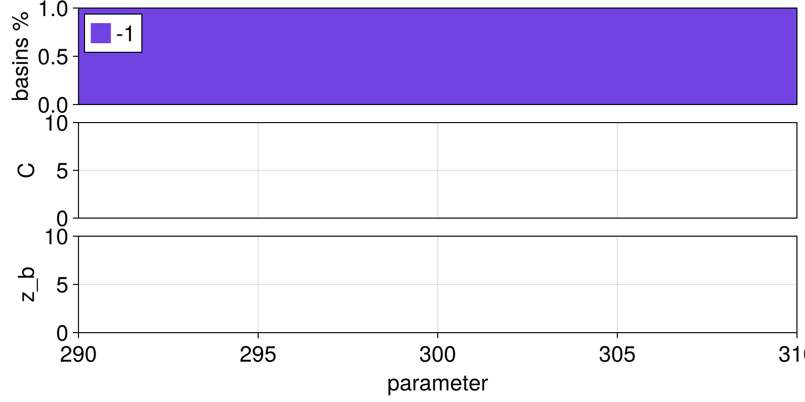

we see for our ad hoc parameterizations, the dynamical system has no stable states for SST > 297. Before that cloud fraction decreases very fast from a Stratocumulus state to a Cumulus one.

The model diverges due to the definition of the entrainment velocity (which is proportional to ΔF_s/Δ₊s) in combination with a fixed s₊: the model reaches a state where Δ₊s is so small that height increases unnaturally well beyond the state space tessellation we defined.