Interactive GUIs, animations, visualizations

Using the functionality of package extensions in Julia v1.9+, DynamicalSystems.jl provides various visualization tools as soon as the Makie package comes into scope (i.e., when using Makie or any of its backends like GLMakie).

The main functionality is interactive_trajectory that allows building custom GUI apps for visualizing the time evolution of dynamical systems. The remaining GUI applications in this page are dedicated to more specialized scenarios.

Interactive- or animated trajectory evolution

The following GUI is obtained with the function interactive_trajectory_timeseries and the code snippet below it!

using DynamicalSystems, GLMakie, ModelingToolkit
# Import canonical time from MTK, however use the unitless version
using ModelingToolkit: t_nounits as t

# Define the variables and parameters in symbolic format
@parameters begin
    a = 0.29
    b = 0.14
    c = 4.52
    d = 1.0
end
@variables begin
    x(t) = 10.0
    y(t) = 0.0
    z(t) = 1.0
    nlt(t) # nonlinear term
end

# Create the equations of the model
eqs = [
    Differential(t)(x) ~ -y - z,
    Differential(t)(y) ~ x + a*y,
    Differential(t)(z) ~ b + nlt - z*c,
    nlt ~ d*z*x, # observed variable
]

# Create the model via ModelingToolkit
@named roessler = ODESystem(eqs, t)
# Do not split parameters so that integer indexing can be used as well
model = structural_simplify(roessler; split = false)
# Cast it into an `ODEProblem` and then into a `DynamicalSystem`.
# Due to low-dimensionality it is preferred to cast into out of place
prob = ODEProblem{false}(model, nothing, (0.0, Inf); u0_constructor = x->SVector(x...))
ds = CoupledODEs(prob)
# If you have "lost" the model, use:
model = referrenced_sciml_model(ds)

# Define which parameters will be interactive during the simulation
parameter_sliders = Dict(
    # can use integer indexing
    1 => 0:0.01:1,
    # the global scope symbol
    b => 0:0.01:1,
    # the symbol obtained from the MTK model
    model.c => 0:0.01:10,
    # or a `Symbol` with same name as the parameter
    # (which is the easiest and recommended way)
    :d => 0.8:0.01:1.2,
)

# Define what variables will be visualized as timeseries
power(u) = sqrt(u[1]*u[1] + u[2]*u[2])
observables = [
    1,         # can use integer indexing
    z,         # MTK state variable (called "unknown")
    model.nlt, # MTK observed variable
    :y,        # `Symbol` instance with same name as symbolic variable
    power,     # arbitrary function of the state
    x^2 - y^2, # arbitrary symbolic expression of symbolic variables
]

# Define what variables will be visualized as state space trajectory
# same as above, any indexing works, but ensure to make the vector `Any`
# so that integers are not converted to symbolic variables
idxs = Any[1, y, 3]

u0s = [
    # we can specify dictionaries, each mapping the variable to its value
    # un-specified variables get the value they currently have in `ds`
    Dict(:x => -4, :y => -4, :z => 0.1),
    Dict(:x => 4, :y => 3, :z => 0.1),
    Dict(:x => -5.72),
    Dict(:x => 5.72, :y => 0.28, :z => 0.21),
]

update_theme!(fontsize = 14)
tail = 1000

fig, dsobs = interactive_trajectory_timeseries(ds, observables, u0s;
    parameter_sliders, Δt = 0.01, tail, idxs,
    figure = (size = (1100, 650),)
)

step!(dsobs, 2tail)

display(fig)

DynamicalSystems.interactive_trajectory_timeseries — Function

interactive_trajectory_timeseries(ds::DynamicalSystem, fs, [, u0s]; kwargs...) → fig, dsobs

Create a Makie Figure to visualize trajectories and timeseries of observables of ds. This Figure can also be used as an interactive GUI to enable interactive control over parameters and time evolution. It can also be used to create videos, as well as customized animations, see below.

fs is a Vector of "indices to observe", i.e., anything that can be given to observe_state. Each observation index will make a timeseries plot. u0s is a Vector of initial conditions. Each is evolved with a unique color and displayed both as a trajectory in state space and as an observed timeseries. Elements of u0 can be either Vector{Real} encoding a full state or Dict to partially set a state from current state of ds (same as in set_state!).

The trajectories from the initial conditions in u0s are all evolved and visualized in parallel. By default only the current state of the system is used. u0s can be anything accepted by a ParallelDynamicalSystem.

Return

Return fig, dsobs::DynamicalSystemObservable. fig is the created Figure. dsobs facilities the creation of custom animations and/or interactive applications, see the custom animations section below.

See also interactive_trajectory.

Interactivity and time stepping keywords

GUI functionality is possible when the plotting backend is GLMakie. Do using GLMakie; GLMakie.activate!() to ensure this is the chosen backend.

add_controls = true: If true, below the state space axis some buttons for animating the trajectories live are added:
- reset: results the parallel trajectories to their initial conditions
- run: when clicked it evolves the trajectories forwards in time indefinitely. click again to stop the evolution.
- step: when clicked it evolves the trajectories forwards in time for the amount of steps chosen by the slider to its right.
The plotted trajectories can always be evolved manually using the custom animations etup that we describe below; add_controls only concerns the buttons and interactivity added to the created figure.
parameter_sliders = nothing: If given, it must be a dictionary, mapping parameter indices (any valid index that can be given to set_parameter!) to ranges of parameter values. Each combination of index and range becomes a slider that can be interactively controlled to alter a system parameter on the fly during time evolution. Below the parameter sliders, three buttons are added for GUI usage:
- update: when clicked the chosen parameter values are propagated into the system
- u.r.s.: when clicked it is equivalent with clicking in order: "update", "reset", "step".
- reset p: when clicked it resets
Parameters can also be altered using the custom animation setup that we describe below; parameter_sliders only conserns the buttons and interactivity added to the created figure.
parameter_names = Dict(keys(ps) .=> string.(keys(ps))): Dictionary mapping parameter keys to labels. Only used if parameter_sliders is given.
Δt: Time step of time evolution. Defaults to 1 for discrete time, 0.01 for continuous time systems. For internal simplicity, continuous time dynamical systems are evolved non-adaptively with constant step size equal to Δt.
pause = nothing: If given, it must be a real number. This number is given to the sleep function, which is called between each plot update. Useful when time integration is computationally inexpensive and animation proceeds too fast.
starting_step = 1: the starting value of the "step" slider.

Visualization keywords

colors: The color for each initial condition (and resulting trajectory and timeseries). Needs to be a Vector of equal length as u0s.
tail = 1000: Length of plotted trajectory (in units of Δt).
fade = 0.5: The trajectories in state space are faded towards full transparency. The alpha channel (transparency) scales as t^fade with t ranging from 0 to 1 (1 being the end of the trajectory). Use fade = 1.0 for linear fading or fade = 0 for no fading. Current default makes fading progress faster at trajectory start and slower at trajectory end.
markersize = 15: Size of markers of trajectory endpoints. For discrete systems half of that is used for the trajectory tail.
plotkwargs = NamedTuple(): A named tuple of keyword arguments propagated to the state space plot (lines for continuous, scatter for discrete systems). plotkwargs can also be a vector of named tuples, in which case each initial condition gets different arguments.

Statespace trajectory keywords

idxs = 1:min(length(u0s[1]), 3): Which variables to plot in a state space trajectory. Any index that can be given to observe_state can be given here.
statespace_axis = true: Whether to create and display an axis for the trajectory plot.
idxs = 1:min(length(u0s[1]), 3): Which variables to plot in a state space trajectory. Any index that can be given to observe_state can be given here. If three indices are given, the trajectory plot is also 3D, otherwise 2D.
lims: A tuple of tuples (min, max) for the axis limits. If not given, they are automatically deduced by evolving each of u0s 1000 Δt units and picking most extreme values (limits are not adjusted by default during the live animations).
figure, axis: both can be named tuples with arbitrary keywords propagated to the generation of the Figure and state space Axis instances.

Timeseries keywords

linekwargs = NamedTuple(): Extra keywords propagated to the timeseries plots. Can also be a vector of named tuples, each one for each unique initial condition.
timeseries_names: A vector of strings with length equal to fs giving names to the y-labels of the timeseries plots.
timeseries_ylims: A vector of 2-tuples for the lower and upper limits of the y-axis of each timeseries plot. If not given it is deduced automatically similarly to lims.
timeunit = 1: the units of time, if any. Sets the units of the timeseries x-axis.
timelabel = "time": label of the x-axis of the timeseries plots.

Custom animations

The second return argument dsobs is a DynamicalSystemObservable. The trajectories plotted in the main panel are linked to observables that are fields of the dsobs. Specifically, the field dsobs.state_obserable is an observable containing the final state of each of the trajectories, i.e., a vector of vectors like u0s. dsobs.param_observable is an observable of the system parameters. These observables are triggered by the interactive GUI buttons (the first two when the system is stepped in time, the last one when the parameters are updated). However, these observables, and hence the corresponding plotted trajectories that are maped from these observables, can be updated via the formal API of DynamicalSystem:

step!(dsobs, n::Int = 1)

will step the system for n steps of Δt time, and only update the plot on the last step. set_parameter!(dsobs, index, value) will update the system parameter and then trigger the parameter observable. Lastly, set_state!(dsobs, new_u [, i]) will set the i-th system state and clear the trajectory plot to the new initial condition.

This information can be used to create custom animations and/or interactive apps. In principle, the only thing a user has to do is create new observables from the existing ones using e.g. the on function and plot these new observables. Various examples are provided in the online documentation.

source

DynamicalSystems.interactive_trajectory — Function

interactive_trajectory(ds::DynamicalSystem [, u0s]; kwargs...) → fig, dsobs

Same as interactive_trajectory_timeseries, but does not plot any timeseries only the trajectory in a (projected) state space.

source

Example 1: interactive trajectory animation

using DynamicalSystems, CairoMakie
F, G, a, b = 6.886, 1.347, 0.255, 4.0
ds = PredefinedDynamicalSystems.lorenz84(; F, G, a, b)

u1 = [0.1, 0.1, 0.1] # periodic
u2 = u1 .+ 1e-3     # fixed point
u3 = [-1.5, 1.2, 1.3] .+ 1e-9 # chaotic
u4 = [-1.5, 1.2, 1.3] .+ 21e-9 # chaotic 2
u0s = [u1, u2, u3, u4]

fig, dsobs = interactive_trajectory(
    ds, u0s; tail = 1000, fade = true,
    idxs = [1,3],
)

fig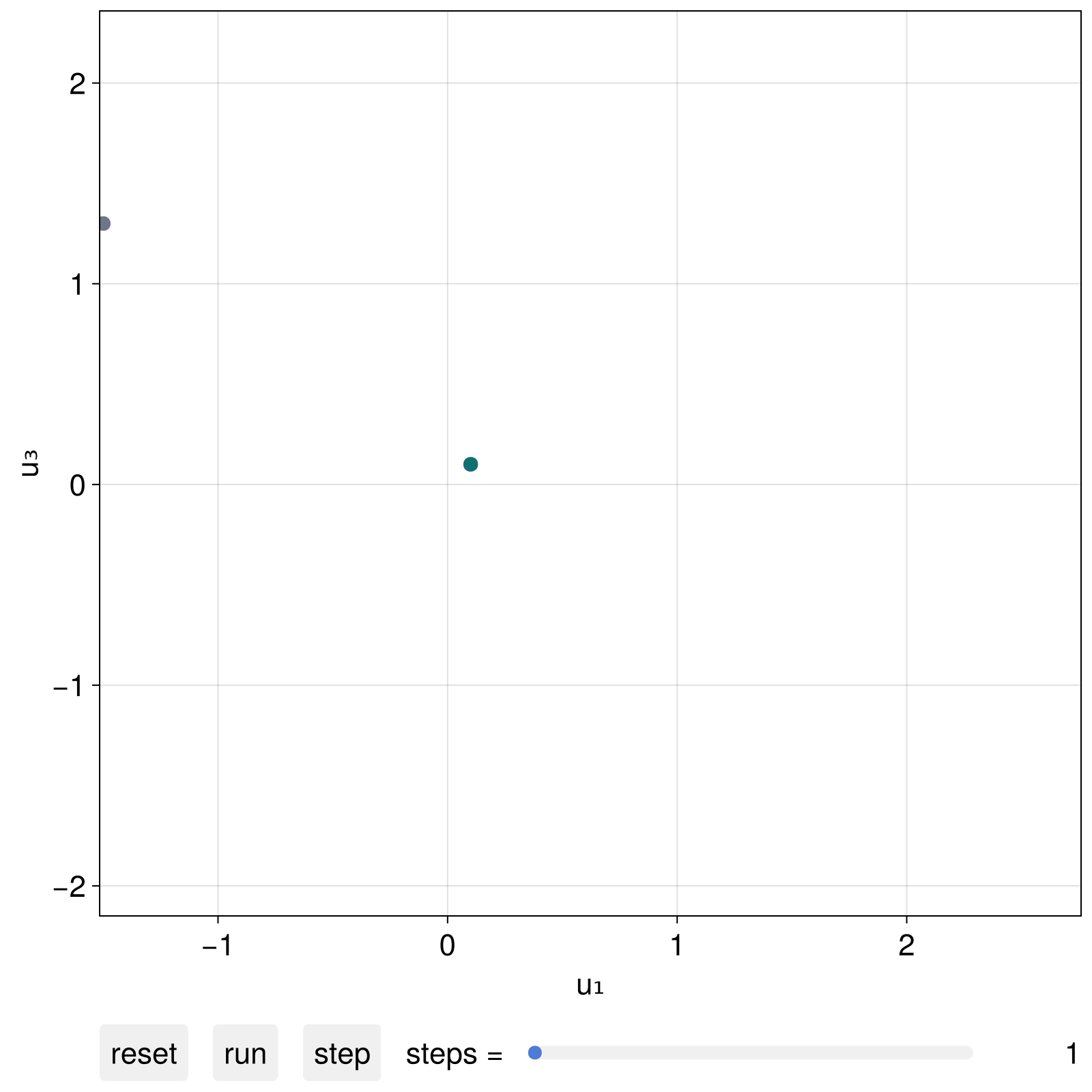

We could interact with this plot live, like in the example video above. We can also progress the visuals via code as instructed by interactive_trajectory utilizing the second returned argument dsobs:

step!(dsobs, 2000)
fig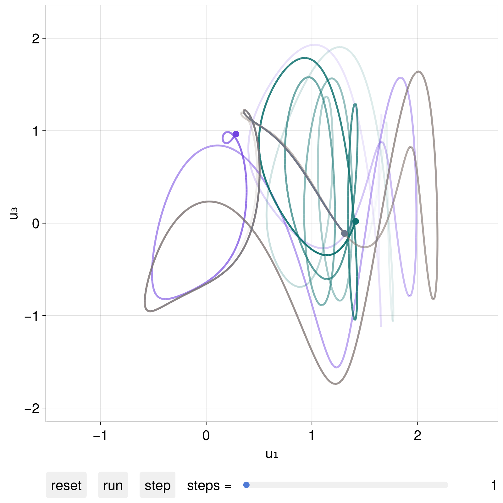

(if you progress the visuals via code you probably want to give add_controls = false as a keyword to interactive_trajectory)

Example 2: Adding parameter-dependent elements to a plot

In this advanced example we add plot elements to the provided figure, and also utilize the parameter observable in dsobs to add animated plot elements that update whenever a parameter updates. The final product of this snippet is in fact the animation at the top of the docstring of interactive_trajectory_panel.

We start with an interactive trajectory panel of the Lorenz63 system, in which we also add sliders for interactively changing parameter values

using DynamicalSystems, CairoMakie

ps = Dict(
    1 => 1:0.1:30,
    2 => 10:0.1:50,
    3 => 1:0.01:10.0,
)
pnames = Dict(1 => "σ", 2 => "ρ", 3 => "β")

lims = ((-30, 30), (-30, 30), (0, 100))

ds = PredefinedDynamicalSystems.lorenz()

u1 = [10,20,40.0]
u3 = [20,10,40.0]
u0s = [u1, u3]

fig, dsobs = interactive_trajectory(
    ds, u0s; parameter_sliders = ps, pnames, lims
)

fig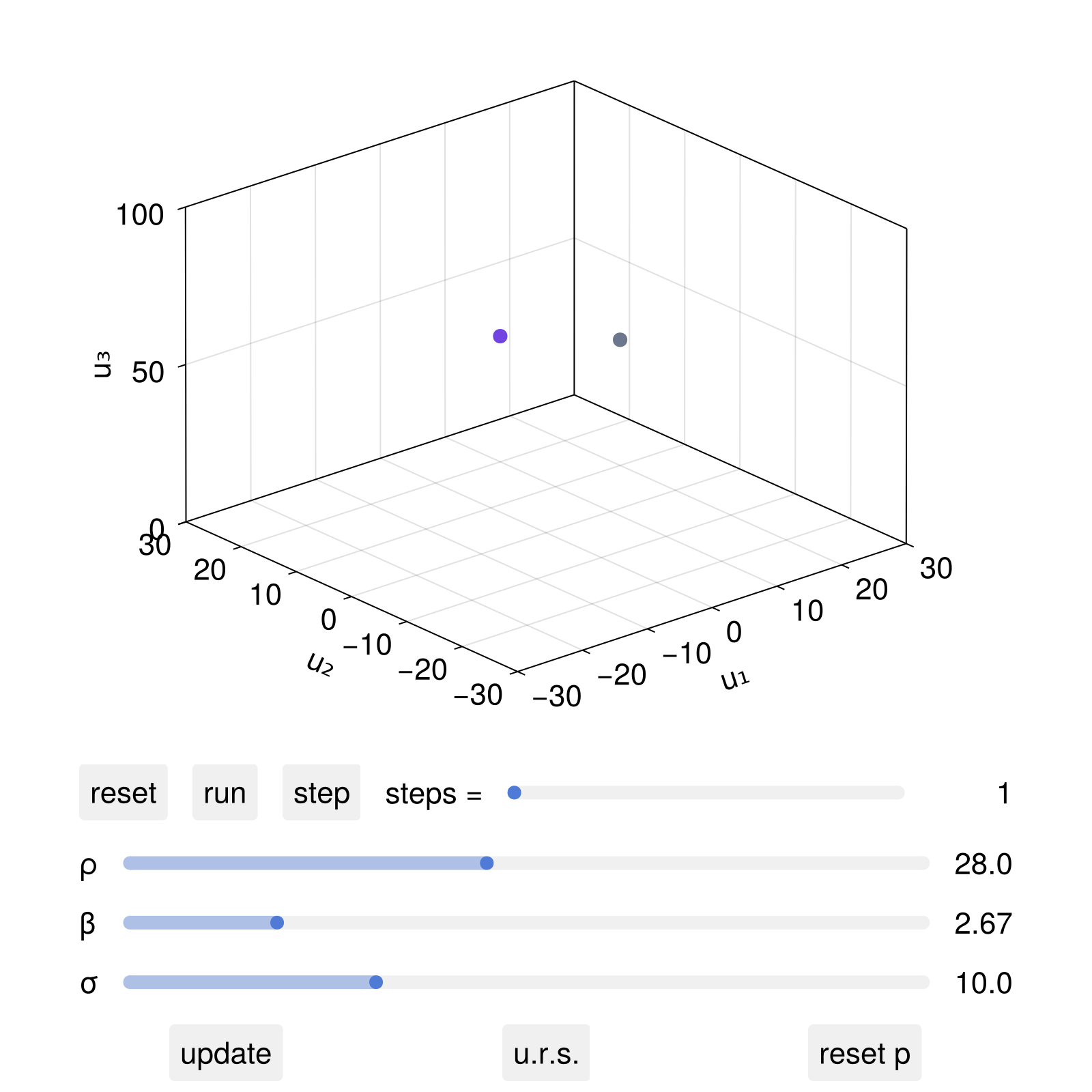

If now one interactively clicked (if using GLMakie) the parameter sliders and then update, the system parameters would be updated accordingly. We can also add new plot elements that depend on the parameter values using the dsobs:

# Fixed points of the lorenz system (without the origin)
lorenz_fixedpoints(ρ,β) = [
    Point3f(sqrt(β*(ρ-1)), sqrt(β*(ρ-1)), ρ-1),
    Point3f(-sqrt(β*(ρ-1)), -sqrt(β*(ρ-1)), ρ-1),
]

# add an observable trigger to the system parameters
fpobs = map(dsobs.param_observable) do params
    σ, ρ, β = params
    return lorenz_fixedpoints(ρ, β)
end

# If we want to plot directly on the trajectory axis, we need to
# extract it from the figure. The first entry of the figure is a grid layout
# containing the axis and the GUI controls. The [1,1] entry of the layout
# is the axis containing the trajectory plot

ax = content(fig[1,1][1,1])
scatter!(ax, fpobs; markersize = 10, marker = :diamond, color = :red)

fig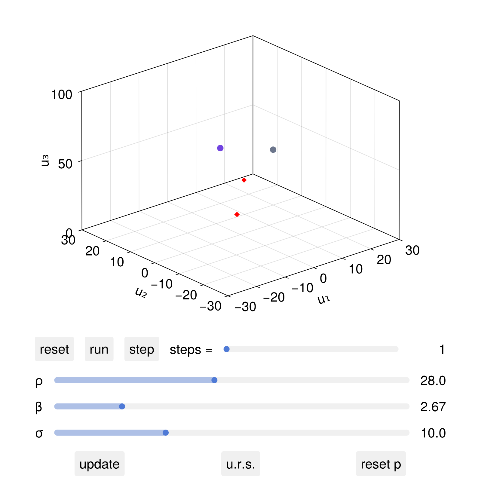

Now, after the live animation "run" button is pressed, we can interactively change the parameter ρ and click update, in which case both the dynamical system's ρ parameter will change, but also the location of the red diamonds.

We can also change the parameters non-interactively using set_parameter!

set_parameter!(dsobs, 2, 50.0)

fig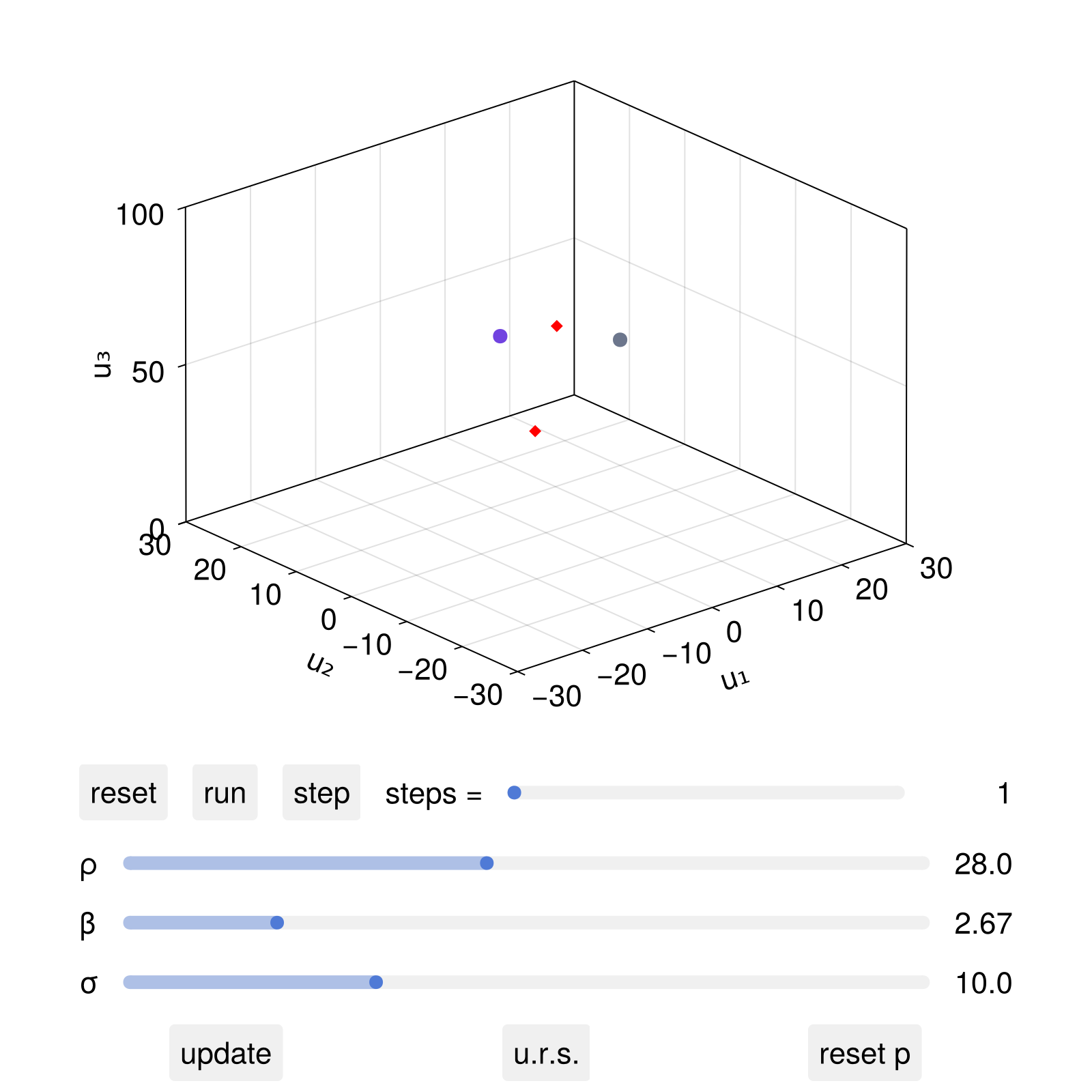

set_parameter!(dsobs, 2, 10.0)

fig

Note that the sliders themselves did not change, as this functionality is for "offline" creation of animations where one doesn't interact with sliders. The keyword add_controls should be given as false in such scenarios.

Example 3: Observed timeseries of the system

using DynamicalSystems, CairoMakie
using LinearAlgebra: norm, dot

# Dynamical system and initial conditions
ds = Systems.thomas_cyclical(b = 0.2)
u0s = [[3, 1, 1.], [1, 3, 1.], [1, 1, 3.]] # must be a vector of states!

# Observables we get timeseries of:
function distance_from_symmetry(u)
    v = SVector{3}(1/√3, 1/√3, 1/√3)
    t = dot(v, u)
    return norm(u - t*v)
end
fs = [3, distance_from_symmetry]

fig, dsobs = interactive_trajectory_timeseries(ds, fs, u0s;
    idxs = [1, 2], Δt = 0.05, tail = 500,
    lims = ((-2, 4), (-2, 4)),
    timeseries_ylims = [(-2, 4), (0, 5)],
    add_controls = false,
    figure = (size = (800, 400),)
)

fig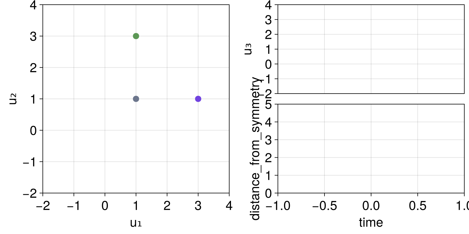

we can progress the simulation:

step!(dsobs, 200)
fig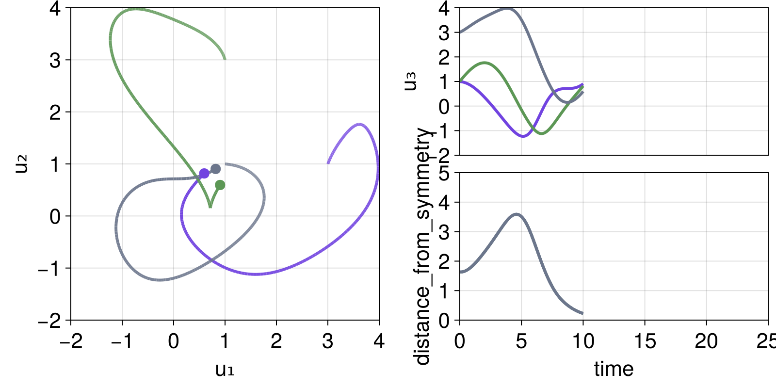

or we can even make a nice video out of it:

record(fig, "thomas_cycl.mp4", 1:100) do i
    step!(dsobs, 10)
end

"thomas_cycl.mp4"

Cobweb Diagrams

DynamicalSystems.interactive_cobweb — Function

interactive_cobweb(ds::DiscreteDynamicalSystem, prange, O::Int = 3; kwargs...)

Launch an interactive application for exploring cobweb diagrams of 1D discrete dynamical systems. Two slides control the length of the plotted trajectory and the current parameter value. The parameter values are obtained from the given prange.

In the cobweb plot, higher order iterates of the dynamic rule f are plotted as well, starting from order 1 all the way to the given order O. Both the trajectory in the cobweb, as well as any iterate f can be turned off by using some of the buttons.

Keywords

fkwargs = [(linewidth = 4.0, color = randomcolor()) for i in 1:O]: plotting keywords for each of the plotted iterates of f
trajcolor = :black: color of the trajectory
pname = "p": name of the parameter slider
pindex = 1: parameter index
xmin = 0, xmax = 1: limits the state of the dynamical system can take
Tmax = 1000: maximum trajectory length
x0s = range(xmin, xmax; length = 101): Possible values for the x0 slider.

source

The animation at the top of this section was done with

using DynamicalSystems, GLMakie

# the second range is a convenience for intermittency example of logistic
rrange = 1:0.001:4.0
# rrange = (rc = 1 + sqrt(8); [rc, rc - 1e-5, rc - 1e-3])

lo = Systems.logistic(0.4; r = rrange[1])
interactive_cobweb(lo, rrange, 5)

Orbit Diagrams

Notice that orbit diagrams and bifurcation diagrams are different things in DynamicalSystems.jl

DynamicalSystems.interactive_orbitdiagram — Function

interactive_orbitdiagram(
    ds::DynamicalSystem, p_index, pmin, pmax, i::Int = 1;
    u0 = nothing, parname = "p", title = ""
)

Open an interactive application for exploring orbit diagrams (ODs) of discrete time dynamical systems. Requires DynamicalSystems.

In essense, the function presents the output of orbitdiagram of the ith variable of the ds, and allows interactively zooming into it.

Keywords control the name of the parameter, the initial state (used for any parameter) or whether to add a title above the orbit diagram.

Interaction

The application is separated in the "OD plot" (left) and the "control panel" (right). On the OD plot you can interactively click and drag with the left mouse button to select a region in the OD. This region is then re-computed at a higher resolution.

The options at the control panel are straight-forward, with

n amount of steps recorded for the orbit diagram (not all are in the zoomed region!)
t transient steps before starting to record steps
d density of x-axis (the parameter axis)
α alpha value for the plotted points.

Notice that at each update n*t*d steps are taken. You have to press update after changing these parameters. Press reset to bring the OD in the original state (and variable). Pressing back will go back through the history of your exploration History is stored when the "update" button is pressed or a region is zoomed in.

You can even decide which variable to get the OD for by choosing one of the variables from the wheel! Because the y-axis limits can't be known when changing variable, they reset to the size of the selected variable.

Accessing the data

What is plotted on the application window is a true orbit diagram, not a plotting shorthand. This means that all data are obtainable and usable directly. Internally we always scale the orbit diagram to [0,1]² (to allow Float64 precision even though plotting is Float32-based). This however means that it is necessary to transform the data in real scale. This is done through the function scaleod which accepts the 5 arguments returned from the current function:

figure, oddata = interactive_orbitdiagram(...)
ps, us = scaleod(oddata)

source

DynamicalSystems.scaleod — Function

scaleod(oddata) -> ps, us

Given the return values of interactive_orbitdiagram, produce orbit diagram data scaled correctly in data units. Return the data as a vector of parameter values and a vector of corresponding variable values.

source

The animation at the top of this section was done with

i = p_index = 1
ds, p_min, p_max, parname = Systems.henon(), 0.8, 1.4, "a"
t = "orbit diagram for the Hénon map"

oddata = interactive_orbitdiagram(ds, p_index, p_min, p_max, i;
                                  parname = parname, title = t)

ps, us = scaleod(oddata)

Interactive Poincaré Surface of Section

DynamicalSystems.interactive_poincaresos — Function

interactive_poincaresos(cds, plane, idxs, complete; kwargs...)

Launch an interactive application for exploring a Poincaré surface of section (PSOS) of the continuous dynamical system cds. Requires DynamicalSystems.

The plane can only be the Tuple type accepted by DynamicalSystems.poincaresos, i.e. (i, r) for the ith variable crossing the value r. idxs gives the two indices of the variables to be displayed, since the PSOS plot is always a 2D scatterplot. I.e. idxs = (1, 2) will plot the 1st versus 2nd variable of the PSOS. It follows that plane[1] ∉ idxs must be true.

complete is a three-argument function that completes the new initial state during interactive use, see below.

The function returns: figure, laststate with the latter being an observable containing the latest initial state.

Keyword Arguments

direction, rootkw : Same use as in DynamicalSystems.poincaresos.
tfinal = (1000.0, 10.0^4) : A 2-element tuple for the range of values for the total integration time (chosen interactively).
color : A function of the system's initial condition, that returns a color to plot the new points with. The color must be RGBf/RGBAf. A random color is chosen by default.
labels = ("u₁" , "u₂") : Scatter plot labels.
scatterkwargs = (): Named tuple of keywords passed to scatter.
diffeq = NamedTuple() : Any extra keyword arguments are passed into init of DiffEq.

Interaction

The application is a standard scatterplot, which shows the PSOS of the system, initially using the system's u0. Two sliders control the total evolution time and the size of the marker points (which is always in pixels).

Upon clicking within the bounds of the scatter plot your click is transformed into a new initial condition, which is further evolved and its PSOS is computed and then plotted into the scatter plot.

Your click is transformed into a full D-dimensional initial condition through the function complete. The first two arguments of the function are the positions of the click on the PSOS. The third argument is the value of the variable the PSOS is defined on. To be more exact, this is how the function is called:

x, y = mouseclick; z = plane[2]
newstate = complete(x, y, z)

The complete function can throw an error for ill-conditioned x, y, z. This will be properly handled instead of breaking the application. This newstate is also given to the function color that gets a new color for the new points.

source

To generate the animation at the start of this section you can run

using InteractiveDynamics, GLMakie, OrdinaryDiffEq, DynamicalSystems
diffeq = (alg = Vern9(), abstol = 1e-9, reltol = 1e-9)

hh = Systems.henonheiles()

potential(x, y) = 0.5(x^2 + y^2) + (x^2*y - (y^3)/3)
energy(x,y,px,py) = 0.5(px^2 + py^2) + potential(x,y)
const E = energy(get_state(hh)...)

function complete(y, py, x)
    V = potential(x, y)
    Ky = 0.5*(py^2)
    Ky + V ≥ E && error("Point has more energy!")
    px = sqrt(2(E - V - Ky))
    ic = [x, y, px, py]
    return ic
end

plane = (1, 0.0) # first variable crossing 0

# Coloring points using the Lyapunov exponent
function λcolor(u)
    λ = lyapunovs(hh, 4000; u0 = u)[1]
    λmax = 0.1
    return RGBf(0, 0, clamp(λ/λmax, 0, 1))
end

state, scene = interactive_poincaresos(hh, plane, (2, 4), complete;
labels = ("q₂" , "p₂"),  color = λcolor, diffeq...)

Scanning a Poincaré Surface of Section

DynamicalSystems.interactive_poincaresos_scan — Function

interactive_poincaresos_scan(A::StateSpaceSet, j::Int; kwargs...)
interactive_poincaresos_scan(As::Vector{StateSpaceSet}, j::Int; kwargs...)

Launch an interactive application for scanning a Poincare surface of section of A like a "brain scan", where the plane that defines the section can be arbitrarily moved around via a slider. Return figure, ax3D, ax2D.

The input dataset must be 3 dimensional, and here the crossing plane is always chosen to be when the j-th variable of the dataset crosses a predefined value. The slider automatically gets all possible values the j-th variable can obtain.

If given multiple datasets, the keyword colors attributes a color to each one, e.g. colors = [JULIADYNAMICS_COLORS[mod1(i, 6)] for i in 1:length(As)].

The keywords linekw, scatterkw are named tuples that are propagated as keyword arguments to the line and scatter plot respectively, while the keyword direction = -1 is propagated to the function DyamicalSystems.poincaresos.

source

The animation at the top of this page was done with

using GLMakie, DynamicalSystems
using OrdinaryDiffEq: Vern9

diffeq = (alg = Vern9(), abstol = 1e-9, reltol = 1e-9)
ds = PredefinedDynamicalSystems.henonheiles()
ds = CoupledODEs(ds, diffeq)

u0s = [
    [0.0, -0.25, 0.42081, 0.0],
    [0.0, 0.1, 0.5, 0.0],
    [0.0, -0.31596, 0.354461, 0.0591255]
]
# inputs
trs = [trajectory(ds, 10000, u0)[1][:, SVector(1,2,3)] for u0 ∈ u0s]
j = 2 # the dimension of the plane

interactive_poincaresos_scan(trs, j; linekw = (transparency = true,))