FractalDimensions.jl
FractalDimensions — Module
FractalDimensions.jl
![]()
![]()
![]()
![]()
A Julia package that estimates various definitions of fractal dimension from data, including so-called "local dimensions and extremal indices" via extreme value theory. It can be used as a standalone package, or as part of DynamicalSystems.jl.
To install it, run import Pkg; Pkg.add("FractalDimensions").
All further information is provided in the documentation, which you can either find online or build locally by running the docs/make.jl file.
Previously, this package was part of ChaosTools.jl.
Publication
FractalDimensions.jl is used in a review article comparing various estimators for fractal dimensions. The paper is likely a relevant read if you are interested in the package. And if you use the package, please cite the paper.
@article{FractalDimensions.jl,
  doi = {10.1063/5.0160394},
  url = {https://doi.org/10.1063/5.0160394},
  year = {2023},
  month = oct,
  publisher = {{AIP} Publishing},
  volume = {33},
  number = {10},
  author = {George Datseris and Inga Kottlarz and Anton P. Braun and Ulrich Parlitz},
  title = {Estimating fractal dimensions: A comparative review and open source implementations},
  journal = {Chaos: An Interdisciplinary Journal of Nonlinear Science}
}Introduction
This package is accompanying a review paper on estimating the fractal dimension: https://arxiv.org/abs/2109.05937. The paper is continuing the discussion of chapter 5 of Nonlinear Dynamics, Datseris & Parlitz, Springer 2022.
There are numerous methods that one can use to calculate a so-called "dimension" of a dataset which in the context of dynamical systems is called the Fractal dimension. One way to do this is to estimate the scaling behaviour of some quantity as a size/scale increases. In the Fractal dimension example below, one finds the scaling of the correlation sum versus a ball radius. In this case, it approximately holds $ \log(C) \approx \Delta\log(\varepsilon) $ for radius $\varepsilon$. The scaling of many other quantities can be estimated as well, such as the generalized entropy, the Higuchi length, or others provided here.
To actually find $\Delta$, one needs to find a linearly scaling region in the graph $\log(C)$ vs. $\log(\varepsilon)$ and estimate its slope. Hence, identifying a linear region is central to estimating a fractal dimension. That is why, the section Linear scaling regions is of central importance for this documentation.
Fractal dimension example
In this simplest example we will calculate the fractal dimension of the chaotic attractor of the Hénon map (for default parameters). For this example, we will generate the data on the spot:
using DynamicalSystemsBase # for simulating dynamical systems
using CairoMakie           # for plotting

henon_rule(x, p, n) = SVector(1.0 - p[1]*x[1]^2 + x[2], p[2]*x[1])
u0 = zeros(2)
p0 = [1.4, 0.3]
henon = DeterministicIteratedMap(henon_rule, u0, p0)

X, t = trajectory(henon, 20_000; Ttr = 100)
scatter(X[:, 1], X[:, 2]; color = ("black", 0.01), markersize = 4)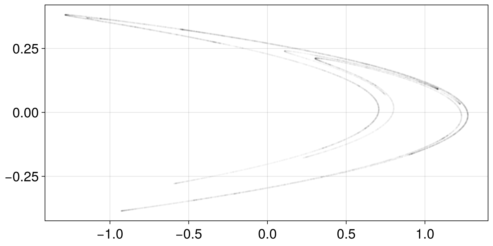
instead of simulating the set X we could load it from disk, e.g., if there was a text file with two columns as x and y coordinates, we would load it as
using DelimitedFiles
file = "path/to/file.csv"
M = readdlm(file)    # here `M` is a matrix with two columns
X = StateSpaceSet(M) # important to convert to a state space set
After we have X, we can start computing a fractal dimension and for this example we will use the correlationsum. Our goal is to compute the correlation sum of X for many different sizes/radii ε. This is as simple as
using FractalDimensions
ες = 2 .^ (-15:0.5:5) # semi-random guess
Cs = correlationsum(X, ες; show_progress = false)
41-element Vector{Float64}:
1.8799060046997648e-6
2.884855757212139e-6
4.514774261286935e-6
7.204639768011599e-6
1.1174441277936103e-5
1.7944102794860256e-5
2.8333583320833955e-5
4.5037748112594364e-5
6.943652817359132e-5
0.0001071696415179241
⋮
0.9486205889705515
0.9999999999999999
0.9999999999999999
0.9999999999999999
0.9999999999999999
0.9999999999999999
0.9999999999999999
0.9999999999999999
0.9999999999999999For a fractal set X dynamical systems theory says that there should be an exponential relationship between the correlation sum and the sizes:
xs = log2.(ες)
ys = log2.(Cs)
scatterlines(xs, ys; axis = (ylabel = L"\log(C_2)", xlabel = L"\log (\epsilon)"))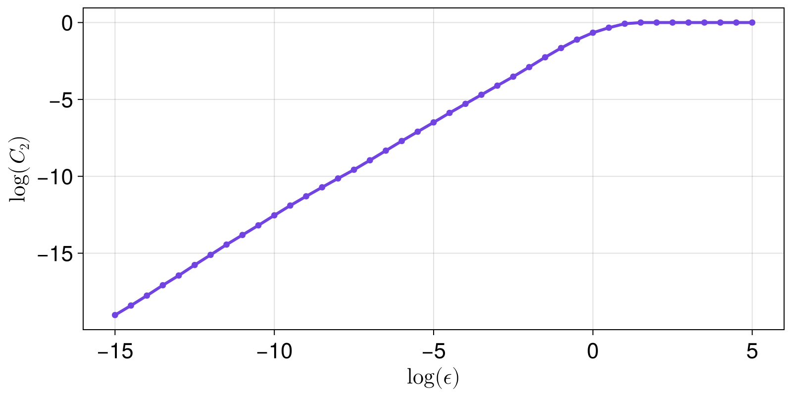
The slope of the linear scaling region of the above plot is the fractal dimension (based on the correlation sum).
Given that we see the plot, we can estimate where the linear scaling region starts and ends. This is generally done using LargestLinearRegion in slopefit. But first, let's visualize what the method does, as it uses linear_regions.
lrs, slopes = linear_regions(xs, ys, tol = 0.25)
fig = Figure()
ax = Axis(fig[1,1]; ylabel = L"\log(C_2)", xlabel = L"\log (\epsilon)")
for r in lrs
    scatterlines!(ax, xs[r], ys[r])
end
fig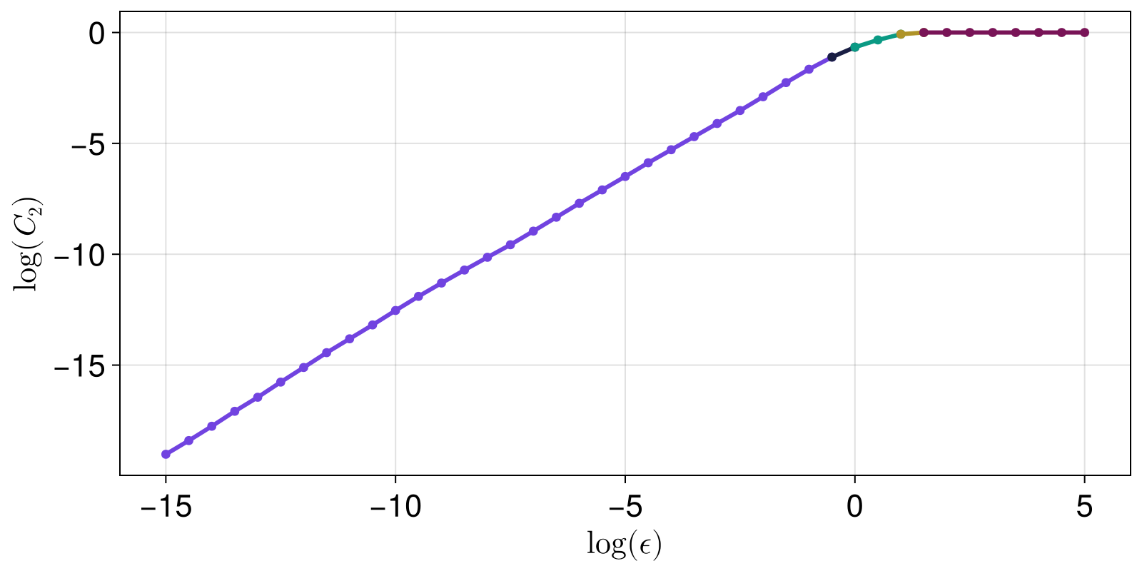
The LargestLinearRegion method finds, and computes the slope of, the largest region:
Δ = slopefit(xs, ys, LargestLinearRegion())(1.2318376178087478, 1.2233720116518771, 1.2403032239656184)This result is an approximation of a fractal dimension.
The whole above pipeline we went through is bundled in grassberger_proccacia_dim. Similar work is done by generalized_dim and many other functions.
As stated clearly by the documentation strings, all pre-made dimension estimating functions (ending in _dim) perform a lot of automated steps, each having its own heuristic choices for function default values. They are more like convenient bundles with on-average good defaults, rather than precise functions. You should be careful when considering the validity of the returned number!
Index (contents)
FractalDimensionsFractalDimensions.AllSlopesDistributionFractalDimensions.BlockMaximaFractalDimensions.ExceedancesFractalDimensions.LargestLinearRegionFractalDimensions.LinearRegressionStateSpaceSets.StateSpaceSetFractalDimensions.boxassisted_correlation_dimFractalDimensions.boxed_correlationsumFractalDimensions.correlationsumFractalDimensions.estimate_boxsizesFractalDimensions.estimate_gev_parametersFractalDimensions.estimate_gpd_parametersFractalDimensions.estimate_r0_buenoorovioFractalDimensions.estimate_r0_theilerFractalDimensions.extremal_index_suevegesFractalDimensions.extremevaltheory_dimFractalDimensions.extremevaltheory_dimsFractalDimensions.extremevaltheory_dims_persistencesFractalDimensions.extremevaltheory_gpdfit_pvaluesFractalDimensions.extremevaltheory_local_dim_persistenceFractalDimensions.fixedmass_correlation_dimFractalDimensions.fixedmass_correlationsumFractalDimensions.generalized_dimFractalDimensions.grassberger_proccacia_dimFractalDimensions.higuchi_dimFractalDimensions.kaplanyorke_dimFractalDimensions.linear_regionFractalDimensions.linear_regionsFractalDimensions.linregFractalDimensions.local_correlation_dimensionFractalDimensions.minimum_pairwise_distanceFractalDimensions.molteno_boxingFractalDimensions.molteno_dimFractalDimensions.pointwise_dimensionsFractalDimensions.prismdim_theilerFractalDimensions.slopefitFractalDimensions.takens_best_estimate_dimStateSpaceSets.standardize
Linear scaling regions
FractalDimensions.slopefit — Function
slopefit(x, y [, t::SLopeFit]; kw...) → s, s05, s95Fit a linear scaling region in the curve of the two AbstractVectors y versus x using t as the estimation method. Return the estimated slope, as well as the confidence intervals for it.
The methods t that can be used for the estimation are:
The keyword ignore_saturation = true ignores saturation that (sometimes) happens at the start and end of the curve y(x), where the curve flattens. The keyword sat_threshold = 0.01 decides what saturation is: while abs(y[i]-y[i+1]) < sat_threshold we are in a saturation regime. Said differently, slopes with value sat_threshold/dx with dx = x[i+1] - x[i] are neglected.
The keyword ci = 0.95 specifies which quantile (and the 1 - quantile) the confidence interval values are returned at, and by defualt it is 95% (and hence also 5%).
FractalDimensions.LinearRegression — Type
LinearRegression <: SlopeFit
LinearRegression()
Standard linear regression fit to all available data. Estimation of the confidence intervals is based om the standard error of the slope following a T-distribution, see:
https://stattrek.com/regression/slope-confidence-interval
FractalDimensions.linreg — Function
linreg(x, y) -> a, bPerform a linear regression to find the best coefficients so that the curve: z = a + b*x has the least squared error with y.
FractalDimensions.LargestLinearRegion — Type
LargestLinearRegion <: SlopeFit
LargestLinearRegion(; dxi::Int = 1, tol = 0.25)
Identify regions where the curve y(x) is linear, by scanning the x-axis every dxi indices sequentially (e.g. at x[1] to x[5], x[5] to x[10], x[10] to x[15] and so on if dxi=5).
If the slope (calculated via linear regression) of a region of width dxi is approximatelly equal to that of the previous region, within relative tolerance tol and absolute tolerance 0, then these two regions belong to the same linear region.
The largest such region is then used to estimate the slope via standard linear regression of all points belonging to the largest linear region. "Largest" here means the region that covers the more extent along the x-axis.
Use linear_regions if you wish to obtain the decomposition into linear regions.
FractalDimensions.linear_regions — Function
linear_regions(x, y; dxi, tol) → lrs, tangentsApply the algorithm described by LargestLinearRegion, and return the indices of x that correspond to the linear regions, lrs, and the tangents at each region (obtained via a second linear regression at each accumulated region). lrs is hence a vector of UnitRanges.
FractalDimensions.linear_region — Function
linear_region(x, y; kwargs...) -> (region, slope)Call linear_regions and identify and return the largest linear region (a UnitRange of the indices of x) and its corresponding slope.
The keywords dxi, tol are propagated as-is to linear_regions. The keyword ignore_saturation = true ignores saturation that (sometimes) happens at the start and end of the curve y(x), where the curve flattens. The keyword sat = 0.01 decides what saturation is (while abs(y[i]-y[i+1])<sat we are in a saturation regime).
The keyword warning = true prints a warning if the linear region is less than 1/3 of the available x-axis.
FractalDimensions.AllSlopesDistribution — Type
AllSlopesDistribution <: SlopeFit
AllSlopesDistribution()
Estimate a slope by computing the distribution of all possible slopes that can be estimated from the curve y(x), according to the method by (Deshmukh et al., 2021). The returned slope is the distribution mean and the confidence intervals are simply the corresponding quantiles of the distribution.
Not implemented yet, the method is here as a placeholder.
FractalDimensions.estimate_boxsizes — Function
estimate_boxsizes(X::AbstractStateSpaceSet; kwargs...) → εsReturn k exponentially spaced values: εs = base .^ range(lower + w, upper + z; length = k), that are a good estimate for sizes ε that are used in calculating a fractal Dimension. It is strongly recommended to standardize input dataset before using this function.
Let d₋ be the minimum pair-wise distance in X, d₋ = dminimum_pairwise_distance(X). Let d₊ be the average total length of X, d₊ = mean(ma - mi) with mi, ma = minmaxima(X). Then lower = log(base, d₋) and upper = log(base, d₊). Because by default w=1, z=-1, the returned sizes are an order of mangitude larger than the minimum distance, and an order of magnitude smaller than the maximum distance.
Keywords
w = 1, z = -1, k = 16: as explained above.base = MathConstants.e: the base used in thelogfunction.warning = true: Print some warnings for bad estimates.autoexpand = true: If the final estimated range does not cover at least 2 orders of magnitude, it is automatically expanded by settingw -= weandz -= ze. You can set different default values to the keywordswe = w, ze = z.
FractalDimensions.minimum_pairwise_distance — Function
minimum_pairwise_distance(X::StateSpaceSet, kdtree = dimension(X) < 10, metric = Euclidean())Return min_d, min_pair: the minimum pairwise distance of all points in the dataset, and the corresponding point pair. The third argument is a switch of whether to use KDTrees or a brute force search.
Generalized (entropy) dimension
Based on the definition of the generalized (Renyi) entropy, one can calculate an appropriate dimension, called generalized dimension:
FractalDimensions.generalized_dim — Function
generalized_dim(X::StateSpaceSet [, sizes]; q = 1, base = 2) -> Δ_qReturn the q order generalized dimension of X, by calculating its histogram-based Rényi entropy for each ε ∈ sizes.
The case of q = 0 is often called "capacity" or "box-counting" dimension, while q = 1 is the "information" dimension.
Description
The returned dimension is approximated by the (inverse) power law exponent of the scaling of the Renyi entropy $H_q$, versus the box size ε, where ε ∈ sizes:
\[H_q \approx -\Delta_q\log_{b}(\varepsilon)\]
$H_q$ is calculated using ComplexityMeasures: Renyi, ValueHistogram, entropy, i.e., by doing a histogram of the data with a given box size.
Calling this function performs a lot of automated steps:
- A vector of box sizes is decided by calling
sizes = estimate_boxsizes(dataset), ifsizesis not given. - For each element of
sizesthe appropriate entropy is calculated as
LetH = [entropy(Renyi(; q, base), ValueHistogram(ε), data) for ε ∈ sizes]x = -log.(sizes). - The curve
H(x)is decomposed into linear regions, usingslopefit(x, h)[1]. - The biggest linear region is chosen, and a fit for the slope of that region is performed using the function
linear_region, which does a simple linear regression fit usinglinreg. This slope is the return value ofgeneralized_dim.
By doing these steps one by one yourself, you can adjust the keyword arguments given to each of these function calls, refining the accuracy of the result. The source code of this function is only 3 lines of code.
This approach to estimating the fractal dimension has been used (to our knowledge) for the first time in (Russell et al., 1980).
FractalDimensions.molteno_dim — Function
molteno_dim(X::AbstractStateSpaceSet; k0::Int = 10, q = 1.0, base = 2)Return an estimate of the generalized_dim of X using the algorithm by (Molteno, 1993). This function is a simple utilization of the probabilities estimated by molteno_boxing so see that function for more details. Here the entropy of the probabilities is computed at each size, and a line is fitted in the entropy vs log(size) graph, just like in generalized_dim.
FractalDimensions.molteno_boxing — Function
molteno_boxing(X::AbstractStateSpaceSet; k0::Int = 10) → (probs, εs)Distribute X into boxes whose size is halved in each step, according to the algorithm by (Molteno, 1993). Division stops if the average number of points per filled box falls below the threshold k0.
Return probs, a vector of Probabilities of finding points in boxes for different box sizes, and the corresponding box sizes εs. These outputs are used in molteno_dim.
Description
Project the data onto the whole interval of numbers that is covered by UInt64. The projected data is distributed into boxes whose size decreases by factor 2 in each step. For each box that contains more than one point 2^D new boxes are created where D is the dimension of the data.
The process of dividing the data into new boxes stops when the number of points over the number of filled boxes falls below k0. The box sizes εs are calculated and returned together with the probs.
This algorithm is faster than the traditional approach of using ValueHistogram(ε::Real), but it is only suited for low dimensional data since it divides each box into 2^D new boxes if D is the dimension. For large D this leads to low numbers of box divisions before the threshold is passed and the divison stops. This results to a low number of data points to fit the dimension to and thereby a poor estimate.
Correlation sum based dimension
FractalDimensions.grassberger_proccacia_dim — Function
grassberger_proccacia_dim(X::AbstractStateSpaceSet, εs = estimate_boxsizes(data); kwargs...)Use the method of Grassberger and Proccacia (Grassberger and Procaccia, 1983), and the correction by (Theiler, 1986), to estimate the correlation dimension Δ_C of X.
This function does something extremely simple:
cm = correlationsum(data, εs; kwargs...)
Δ_C = slopefit(rs, ys)(log2.(sizes), log2.(cm))[1]
i.e. it calculates correlationsum for various radii and then tries to find a linear region in the plot of the log of the correlation sum versus log(ε).
See correlationsum for the available keywords. See also takens_best_estimate_dim, boxassisted_correlation_dim.
FractalDimensions.correlationsum — Function
correlationsum(X, ε::Real; w = 0, norm = Euclidean(), q = 2) → C_q(ε)Calculate the q-order correlation sum of X (StateSpaceSet or timeseries) for a given radius ε and norm. They keyword show_progress = true can be used to display a progress bar for large X.
correlationsum(X, εs::AbstractVector; w, norm, q) → C_q(ε)If εs is a vector, C_q is calculated for each ε ∈ εs more efficiently. Multithreading is also enabled over the available threads (Threads.nthreads()). The function boxed_correlationsum is typically faster if the dimension of X is small and if maximum(εs) is smaller than the size of X.
Keyword arguments
q = 2: order of the correlation sumnorm = Euclidean(): distance normw = 0: Theiler windowshow_progress = true: display a progress bar
Description
The correlation sum is defined as follows for q=2:
\[C_2(\epsilon) = \frac{2}{(N-w)(N-w-1)}\sum_{i=1}^{N}\sum_{j=1+w+i}^{N} B(||X_i - X_j|| < \epsilon)\]
for as follows for q≠2
\[C_q(\epsilon) = \left[ \sum_{i=1}^{N} \alpha_i \left[\sum_{j:|i-j| > w} B(||X_i - X_j|| < \epsilon)\right]^{q-1}\right]^{1/(q-1)}\]
where
\[\alpha_i = 1 / (N (\max(N-w, i) - \min(w + 1, i))^{(q-1)})\]
with $N$ the length of X and $B$ gives 1 if its argument is true. w is the Theiler window.
See the article of Grassberger for the general definition (Grassberger, 2007) and the book "Nonlinear Time Series Analysis" (Kantz and Schreiber, 2003), Ch. 6, for a discussion around choosing best values for w, and Ch. 11.3 for the explicit definition of the q-order correlationsum. Note that the formula in 11.3 is incorrect, but corrected here, indices are adapted to take advantage of all available points and also note that we immediatelly exponentiate $C_q$ to $1/(q-1)$, so that it scales exponentially as $C_q \propto \varepsilon ^\Delta_q$ versus the size $\varepsilon$.
Box-assisted version
FractalDimensions.boxassisted_correlation_dim — Function
boxassisted_correlation_dim(X::AbstractStateSpaceSet; kwargs...)Use the box-assisted optimizations of (Bueno-Orovio and Pérez-Garcı́a, 2007) to estimate the correlation dimension Δ_C of X.
This function does something extremely simple:
εs, Cs = boxed_correlationsum(X; kwargs...)
slopefit(log2.(εs), log2.(Cs))[1]
and hence see boxed_correlationsum for more information and available keywords.
FractalDimensions.boxed_correlationsum — Function
boxed_correlationsum(X::AbstractStateSpaceSet, εs, r0 = maximum(εs); kwargs...) → CsEstimate the correlationsum for each size ε ∈ εs using an optimized algorithm that first distributes data into boxes of size r0, and then computes the correlation sum for each box and each neighboring box of each box. This method is much faster than correlationsum, provided that the box size r0 is significantly smaller than the attractor length. Good choices for r0 are estimate_r0_buenoorovio or estimate_r0_theiler.
boxed_correlationsum(X::AbstractStateSpaceSet; kwargs...) → εs, CsIn this method the minimum inter-point distance and estimate_r0_buenoorovio of X are used to estimate suitable εs for the calculation, which are also returned.
Keyword arguments
q = 2: The order of the correlation sum.P = 2: The prism dimension.w = 0: The Theiler window.show_progress = false: Whether to display a progress bar for the calculation.norm = Euclidean(): Distance norm.
Description
C_q(ε) is calculated for every ε ∈ εs and each of the boxes to then be summed up afterwards. The method of splitting the data into boxes was implemented according to (Theiler, 1987). w is the Theiler window. P is the prism dimension. If P is unequal to the dimension of the data, only the first P dimensions are considered for the box distribution (this is called the prism-assisted version). By default P is 2, which is the version suggested by [Bueno2007]. Alternative for P is the prismdim_theiler. Note that only when P = dimension(X) the boxed version is guaranteed to be exact to the original correlationsum. For any other P, some point pairs that should have been included may be skipped due to having smaller distance in the remaining dimensions, but larger distance in the first P dimensions.
FractalDimensions.prismdim_theiler — Function
prismdim_theiler(X)An algorithm to find the ideal choice of a prism dimension for boxed_correlationsum using Theiler's original suggestion.
FractalDimensions.estimate_r0_buenoorovio — Function
estimate_r0_buenoorovio(X::AbstractStateSpaceSet, P = 2) → r0, ε0Estimate a reasonable size for boxing X, proposed by Bueno-Orovio and Pérez-García (Bueno-Orovio and Pérez-Garcı́a, 2007), before calculating the correlation dimension as presented by (Theiler, 1987). Return the size r0 and the minimum interpoint distance ε0 in the data.
If instead of boxes, prisms are chosen everything stays the same but P is the dimension of the prism. To do so the dimension ν is estimated by running the algorithm by Grassberger and Procaccia (Grassberger and Procaccia, 1983) with √N points where N is the number of total data points. An effective size ℓ of the attractor is calculated by boxing a small subset of size N/10 into boxes of sidelength r_ℓ and counting the number of filled boxes η_ℓ.
\[\ell = r_\ell \eta_\ell ^{1/\nu}\]
The optimal number of filled boxes η_opt is calculated by minimising the number of calculations.
\[\eta_\textrm{opt} = N^{2/3}\cdot \frac{3^\nu - 1}{3^P - 1}^{1/2}.\]
P is the dimension of the data or the number of edges on the prism that don't span the whole dataset.
Then the optimal boxsize $r_0$ computes as
\[r_0 = \ell / \eta_\textrm{opt}^{1/\nu}.\]
FractalDimensions.estimate_r0_theiler — Function
estimate_r0_theiler(X::AbstractStateSpaceSet) → r0, ε0Estimate a reasonable size for boxing the data X before calculating the boxed_correlationsum proposed by (Theiler, 1987). Return the boxing size r0 and minimum inter-point distance in X, ε0.
To do so the dimension is estimated by running the algorithm by Grassberger and Procaccia (Grassberger and Procaccia, 1983) with √N points where N is the number of total data points. Then the optimal boxsize $r_0$ computes as
\[r_0 = R (2/N)^{1/\nu}\]
where $R$ is the size of the chaotic attractor and $\nu$ is the estimated dimension.
Fixed mass correlation sum
FractalDimensions.fixedmass_correlation_dim — Function
fixedmass_correlation_dim(X [, max_j]; kwargs...)Use the fixed mass algorithm for computing the correlation sum, and use the result to compute the correlation dimension Δ_M of X.
This function does something extremely simple:
rs, ys = fixedmass_correlationsum(X, args...; kwargs...)
slopefit(rs, ys)[1]FractalDimensions.fixedmass_correlationsum — Function
fixedmass_correlationsum(X [, max_j]; metric = Euclidean(), M = length(X)) → rs, ysA fixed mass algorithm for the calculation of the correlationsum, and subsequently a fractal dimension $\Delta$, with max_j the maximum number of neighbours that should be considered for the calculation.
By default max_j = clamp(N*(N-1)/2, 5, 32) with N the data length.
Keyword arguments
Mdefines the number of points considered for the averaging of distances, randomly subsampling them fromX.metric = Euclidean()is the distance metric.start_j = 4computes the equation below starting fromj = start_j. Typically the firstjvalues have not converged to the correct scaling of the fractal dimension.
Description
"Fixed mass" algorithms mean that instead of trying to find all neighboring points within a radius, one instead tries to find the max radius containing j points. A correlation sum is obtained with this constrain, and equivalently the mean radius containing k points. Based on this, one can calculate $\Delta$ approximating the information dimension. The implementation here is due to to (Grassberger, 1988), which defines
\[Ψ(j) - \log N \sim \Delta \times \overline{\log \left( r_{(j)}\right)}\]
where $\Psi(j) = \frac{\text{d} \log Γ(j)}{\text{d} j}$ is the digamma function, rs = $\overline{\log \left( r_{(j)}\right)}$ is the mean logarithm of a radius containing j neighboring points, and ys = $\Psi(j) - \log N$ ($N$ is the length of the data). The amount of neighbors found $j$ range from 2 to max_j. The numbers are also converted to base $2$ from base $e$.
$\Delta$ can be computed by using linear_region(rs, ys).
Takens best estimate
FractalDimensions.takens_best_estimate_dim — Function
takens_best_estimate_dim(X, εmax, metric = Chebyshev(), εmin = 0)Use the "Takens' best estimate" [Takens1985][Theiler1988] method for estimating the correlation dimension.
The original formula is
\[\Delta_C \approx \frac{C(\epsilon_\text{max})}{\int_0^{\epsilon_\text{max}}(C(\epsilon) / \epsilon) \, d\epsilon}\]
where $C$ is the correlationsum and $\epsilon_\text{max}$ is an upper cutoff. Here we use the later expression
\[\Delta_C \approx - \frac{1}{\eta},\quad \eta = \frac{1}{(N-1)^*}\sum_{[i, j]^*}\log(||X_i - X_j|| / \epsilon_\text{max})\]
where the sum happens for all $i, j$ so that $i < j$ and $||X_i - X_j|| < \epsilon_\text{max}$. In the above expression, the bias in the original paper has already been corrected, as suggested in [Borovkova1999].
According to [Borovkova1999], introducing a lower cutoff εmin can make the algorithm more stable (no divergence), this option is given but defaults to zero.
If X comes from a delay coordinates embedding of a timseries x, a recommended value for $\epsilon_\text{max}$ is std(x)/4.
You may also use
Δ_C, Δu_C, Δl_C = FractalDimensions.takens_best_estimate(args...)to obtain the upper and lower 95% confidence intervals. The intervals are estimated from the log-likelihood function by finding the values of Δ_C where the function has fallen by 2 from its maximum, see e.g. [Barlow] chapter 5.3.
Pointwise (local) correlation dimensions
FractalDimensions.pointwise_dimensions — Function
pointwise_dimensions(X::StateSpaceSet, εs::AbstractVector; kw...) → ΔlocReturn the pointwise dimensions for each point in X, i.e., the exponential scaling of the inner correlation sum
\[c_q(\epsilon) = \left[\sum_{j:|i-j| > w} B(||X_i - X_j|| < \epsilon)\right]^{q-1}\]
versus $\epsilon$. Δloc[i] is the exponential scaling (deduced by a call to linear_region) of $c_q$ versus $\epsilon$ for the ith point of X.
Keywords are the same as in correlationsum. To obtain the inner correlation sums without doing the exponential scaling fit use FractalDimensions.pointwise_correlationsums with same inputs.
FractalDimensions.local_correlation_dimension — Function
local_correlation_dimension(X, ζ [, εs]; kw...) → Δ_ζReturn the local dimension Δ_ζ around state space point ζ given a set of state space points X which is assumed to surround (or be sufficiently near to) ζ. The local dimension is the exponential scaling of the correlation sum for point ζ versus some radii εs. εs can be a vector of reals, or it can be an integer, in which space that many points are equi-spaced logarithmically between the minimum and maximum distance of X to ζ.
Keyword arguments
q = 2, norm = Euclidean(): same as incorrelationsum.fit = LinearRegression(): given toslopefitto estimate the dimension. This default assumes that the setXis already sufficiently close toζ.
Kaplan-Yorke dimension
FractalDimensions.kaplanyorke_dim — Function
kaplanyorke_dim(λs::AbstractVector)Calculate the Kaplan-Yorke dimension, a.k.a. Lyapunov dimension (Kaplan and Yorke, 1979) from the given Lyapunov exponents λs.
Description
The Kaplan-Yorke dimension is simply the point where cumsum(λs) becomes zero (interpolated):
\[ D_{KY} = k + \frac{\sum_{i=1}^k \lambda_i}{|\lambda_{k+1}|},\quad k = \max_j \left[ \sum_{i=1}^j \lambda_i > 0 \right].\]
If the sum of the exponents never becomes negative the function will return the length of the input vector.
Useful in combination with lyapunovspectrum from ChaosTools.jl.
Higuchi dimension
FractalDimensions.higuchi_dim — Function
higuchi_dim(x::AbstractVector [, ks])Estimate the Higuchi dimension (Higuchi, 1988) of the graph of x.
Description
The Higuchi dimension is a number Δ ∈ [1, 2] that quantifies the roughness of the graph of the function x(t), assuming here that x is equi-sampled, like in the original paper.
The method estimates how the length of the graph increases as a function of the indices difference (which, in this context, is equivalent with differences in t). Specifically, we calculate the average length versus k as
\[L_m(k) = \frac{N-1}{\lfloor \frac{N-m}{k} \rfloor k^2} \sum_{i=1}^{\lfloor \frac{N-m}{k} \rfloor} |X_N(m+ik)-X_N(m+(i-1)k)| \\ L(k) = \frac{1}{k} \sum_{m=1}^k L_m(k)\]
and then use linear_region in -log2.(k) vs log2.(L) as per usual when computing a fractal dimension.
The algorithm chooses default ks to be exponentially spaced in base-2, up to at most 2^8. A user can provide their own ks as a second argument otherwise.
Use FractalDimensions.higuchi_length(x, ks) to obtain $L(k)$ directly.
Extreme value value theory dimensions
The central function for this is extremevaltheory_dims_persistences which utilizes either Exceedances or BlockMaxima.
Main functions
FractalDimensions.extremevaltheory_dims_persistences — Function
extremevaltheory_dims_persistences(x::AbstractStateSpaceSet, est; kwargs...)Return the local dimensions Δloc and the persistences θloc for each point in the given set according to extreme value theory (Lucarini et al., 2016). The type of est decides which approach to use when computing the dimension. The possible estimators are:
The computation is parallelized to available threads (Threads.nthreads()).
See also extremevaltheory_gpdfit_pvalues for obtaining confidence on the results.
Keyword arguments
show_progress = true: displays a progress bar.compute_persistence = true:whether to aso compute local persistencesθloc(also called extremal indices). Iffalse,θlocareNaNs.
FractalDimensions.extremevaltheory_dim — Function
extremevaltheory_dim(X::StateSpaceSet, p; kwargs...) → ΔConvenience syntax that returns the mean of the local dimensions of extremevaltheory_dims_persistences with X, p.
FractalDimensions.extremevaltheory_dims — Function
extremevaltheory_dims(X::StateSpaceSet, p; kwargs...) → ΔlocConvenience syntax that returns the local dimensions of extremevaltheory_dims_persistences with X, p.
FractalDimensions.extremevaltheory_local_dim_persistence — Function
extremevaltheory_local_dim_persistence(X::StateSpaceSet, ζ, p; kw...)Return the local values Δ, θ of the fractal dimension and persistence of X around a state space point ζ. p and kw are as in extremevaltheory_dims_persistences.
FractalDimensions.extremal_index_sueveges — Function
extremal_index_sueveges(y::AbstractVector, p)Compute the extremal index θ of y through the Süveges formula for quantile probability p, using the algorithm of (Süveges, 2007).
Exceedances estimator
FractalDimensions.Exceedances — Type
Exceedances(p::Real, estimator::Symbol)Instructions type for extremevaltheory_dims_persistences and related functions. This method sets a threshold and fits the exceedances to Generalized Pareto Distribution (GPD). The parameter p is a number between 0 and 1 that determines the p-quantile for the threshold and computation of the extremal index. The argument estimator is a symbol that decides how the GPD is fitted to the data. It can take the values :exp, :pwm, :mm, as in estimate_gpd_parameters.
Description
For each state space point $\mathbf{x}_i$ in X we compute $g_i = -\log(||\mathbf{x}_i - \mathbf{x}_j|| ) \; \forall j = 1, \ldots, N$ with $||\cdot||$ the Euclidean distance. Next, we choose an extreme quantile probability $p$ (e.g., 0.99) for the distribution of $g_i$. We compute $g_p$ as the $p$-th quantile of $g_i$. Then, we collect the exceedances of $g_i$, defined as $E_i = \{ g_i - g_p: g_i \ge g_p \}$, i.e., all values of $g_i$ larger or equal to $g_p$, also shifted by $g_p$. There are in total $n = N(1-q)$ values in $E_i$. According to extreme value theory, in the limit $N \to \infty$ the values $E_i$ follow a two-parameter Generalized Pareto Distribution (GPD) with parameters $\sigma,\xi$ (the third parameter $\mu$ of the GPD is zero due to the positive-definite construction of $E$). Within this extreme value theory approach, the local dimension $\Delta^{(E)}_i$ assigned to state space point $\textbf{x}_i$ is given by the inverse of the $\sigma$ parameter of the GPD fit to the data[Lucarini2012], $\Delta^{(E)}_i = 1/\sigma$. $\sigma$ is estimated according to the estimator keyword.
A more precise description of this process is given in the review paper (Datseris et al., 2023).
FractalDimensions.estimate_gpd_parameters — Function
estimate_gpd_parameters(X::AbstractVector{<:Real}, estimator::Symbol)Estimate and return the parameters σ, ξ of a Generalized Pareto Distribution fit to X (which typically is the exceedances of the log distance of a state space set), assuming that minimum(X) ≥ 0 and hence the parameter μ is 0 (if not, simply shift X by its minimum), according to the methods provided in (Pons et al., 2023).
The estimator can be:
:exp: Assume the distribution is exponential instead of GP and getσfrom mean ofXand setξ = 0.mm: Standing for "method of moments", estimants are given by\[\xi = (\bar{x}^2/s^2 - 1)/2, \quad \sigma = \bar{x}(\bar{x}^2/s^2 + 1)/2\]
with $\bar{x}$ the sample mean and $s^2$ the sample variance. This estimator only exists if the true distributionξvalue is < 0.5.
FractalDimensions.extremevaltheory_gpdfit_pvalues — Function
extremevaltheory_gpdfit_pvalues(X, p; kw...)Return various computed quantities that may quantify the significance of the results of extremevaltheory_dims_persistences(X, p; kw...), terms of quantifying how well a Generalized Pareto Distribution (GPD) describes exceedences in the input data.
Keyword arguments
show_progress = true: display a progress bar.TestType = ApproximateOneSampleKSTest: the test type to use. It can beApproximateOneSampleKSTest, ExactOneSampleKSTest, CramerVonMises. We noticed thatOneSampleADTestsometimes yielded nonsensical results: all p-values were equal and were very small ≈ 1e-6.nbins = round(Int, length(X)*(1-p)/20): number of bins to use when computing the histogram of the exceedances for computing the NRMSE. The default value will use equally spaced bins that are equal to the length of the exceedances divided by 20.
Description
The function computes the exceedances $E_i$ for each point $x_i \in X$ as in extremevaltheory_dims_persistences. It returns 5 quantities, all being vectors of length length(X):
Es, all exceedences, as a vector of vectors.sigmas, xisthe fitted σ, ξ to the GPD fits for each exceedancenrmsesthe normalized root mean square distance of the fitted GPD to the histogram of the exceedancespvaluesthe pvalues of a statistical test of the appropriateness of the GPD fit
The output nrmses quantifies the distance between the fitted GPD and the empirical histogram of the exceedances. It is computed as
\[NRMSE = \sqrt{\frac{\sum{(P_j - G_j)^2}{\sum{(P_j - U)^2}}\]
where $P_j$ the empirical (observed) probability at bin $j$, $G_j$ the fitted GPD probability at the midpoint of bin $j$, and $U$ same as $G_j$ but for the uniform distribution. The divisor of the equation normalizes the expression, so that the error of the empirical distribution is normalized to the error of the empirical distribution with fitting it with the uniform distribution. It is expected that NRMSE < 1. The smaller it is, the better the data are approximated by GPD versus uniform distribution.
The output pvalues is a vector of p-values. pvalues[i] corresponds to the p-value of the hypothesis: "The exceedences around point X[i] are sampled from a GPD" versus the alternative hypothesis that they are not. To extract the p-values, we perform a one-sample hypothesis via HypothesisTests.jl to the fitted GPD. Very small p-values then indicate that the hypothesis should be rejected and the data are not well described by a GPD. This can be an indication that we do not have enough data, or that we choose too high of a quantile probability p, or that the data are not suitable in general. This p-value based method for significance has been used in [Faranda2017], but it is unclear precisely how it was used.
For more details on how these quantities may quantify significance, see our review paper.
Block-maxima estimator
FractalDimensions.BlockMaxima — Type
BlockMaxima(blocksize::Int, p::Real)Instructions type for extremevaltheory_dims_persistences and related functions. This method divides the input data into blocks of length blocksize and fits the maxima of each block to a Generalized Extreme Value distribution. In order for this method to work correctly, both the blocksize and the number of blocks must be high. Note that there are data points that are not used by the algorithm. Since it is not always possible to express the number of input data poins as N = blocksize * nblocks + 1. To reduce the number of unused data, chose an N equal or superior to blocksize * nblocks + 1. This method and several variants of it has been studied in (Faranda et al., 2011)
The parameter p is a number between 0 and 1 that determines the p-quantile for the computation of the extremal index and hence is irrelevant if compute_persistences = false in extremevaltheory_dims_persistences.
See also estimate_gev_parameters.
FractalDimensions.estimate_gev_parameters — Function
estimate_gev_parameters(X::AbstractVector{<:Real}, θ::Real)Estimate and return the parameters σ, μ of a Generalized Extreme Value distribution fit to X (which typically is the collected block maxima of the log distances of a state space set), assuming that the parameter ξ is 0, and that the extremal index θ is a known constant, and can be estimated through the function extremal_index_sueveges. The estimators through the method of moments are given by σ = √((̄x²-̄x^2)/(π^2/6)) μ = ̄x - σ(log(θ) + γ) where γ is the constant of Euler-Mascheroni.
Theiler window
The Theiler window is a concept that is useful when finding neighbors in a dataset that is coming from the sampling of a continuous dynamical system. Itt tries to eliminate spurious "correlations" (wrongly counted neighbors) due to a potentially dense sampling of the trajectory. Typically a good choice for w coincides with the choice an optimal delay time, see DelayEmbeddings.estimate_delay, for any of the timeseries of the dataset.
For more details, see Chapter 5 of Nonlinear Dynamics, Datseris & Parlitz, Springer 2022.
StateSpaceSet reference
StateSpaceSets.StateSpaceSet — Type
StateSpaceSet{D, T, V} <: AbstractVector{V}A dedicated interface for sets in a state space. It is an ordered container of equally-sized points of length D, with element type T, represented by a vector of type V. Typically V is SVector{D,T} or Vector{T} and the data are always stored internally as Vector{V}. SSSet is an alias for StateSpaceSet.
The underlying Vector{V} can be obtained by vec(ssset), although this is almost never necessary because StateSpaceSet subtypes AbstractVector and extends its interface. StateSpaceSet also supports almost all sensible vector operations like append!, push!, hcat, eachrow, among others. When iterated over, it iterates over its contained points.
Construction
Constructing a StateSpaceSet is done in three ways:
- By giving in each individual columns of the state space set as
Vector{<:Real}:StateSpaceSet(x, y, z, ...). - By giving in a matrix whose rows are the state space points:
StateSpaceSet(m). - By giving in directly a vector of vectors (state space points):
StateSpaceSet(v_of_v).
All constructors allow for two keywords:
containerwhich sets the type ofV(the type of inner vectors). At the moment options are onlySVector,MVector, orVector, and by defaultSVectoris used.nameswhich can be an iterable of lengthDwhose elements areSymbols. This allows assigning a name to each dimension and accessing the dimension by name, see below.namesisnothingif not given. UseStateSpaceSet(s; names)to add names to an existing sets.
Description of indexing
When indexed with 1 index, StateSpaceSet behaves exactly like its encapsulated vector. i.e., a vector of vectors (state space points). When indexed with 2 indices it behaves like a matrix where each row is a point.
In the following let i, j be integers, typeof(X) <: AbstractStateSpaceSet and v1, v2 be <: AbstractVector{Int} (v1, v2 could also be ranges, and for performance benefits make v2 an SVector{Int}).
X[i] == X[i, :]gives theith point (returns anSVector)X[v1] == X[v1, :], returns aStateSpaceSetwith the points in those indices.X[:, j]gives thejth variable timeseries (or collection), asVectorX[v1, v2], X[:, v2]returns aStateSpaceSetwith the appropriate entries (first indices being "time"/point index, while second being variables)X[i, j]value of thejth variable, at theith timepoint
In all examples above, j can also be a Symbol, provided that names has been given when creating the state space set. This allows accessing a dimension by name. This is provided as a convenience and it is not an optimized operation, hence recommended to be used primarily with X[:, j::Symbol].
Use Matrix(ssset) or StateSpaceSet(matrix) to convert. It is assumed that each column of the matrix is one variable. If you have various timeseries vectors x, y, z, ... pass them like StateSpaceSet(x, y, z, ...). You can use columns(dataset) to obtain the reverse, i.e. all columns of the dataset in a tuple.
StateSpaceSets.standardize — Function
standardize(d::StateSpaceSet) → rCreate a standardized version of the input set where each column is transformed to have mean 0 and standard deviation 1.
standardize(x::AbstractVector{<:Real}) = (x - mean(x))/std(x)References
- Bueno-Orovio, A. and Pérez-Garcı́a, V. M. (2007). Enhanced box and prism assisted algorithms for computing the correlation dimension. Chaos, Solitons &$\mathsemicolon$ Fractals 34, 509–518.
- Datseris, G.; Kottlarz, I.; Braun, A. P. and Parlitz, U. (2023). Estimating fractal dimensions: A comparative review and open source implementations. Chaos: An Interdisciplinary Journal of Nonlinear Science 33.
- Deshmukh, V.; Bradley, E.; Garland, J. and Meiss, J. D. (2021). Toward automated extraction and characterization of scaling regions in dynamical systems. Chaos: An Interdisciplinary Journal of Nonlinear Science 31.
- Faranda, D.; Lucarini, V.; Turchetti, G. and Vaienti, S. (2011). Numerical convergence of the block-maxima approach to the generalized extreme value distribution. Journal of statistical physics 145, 1156–1180.
- Grassberger, P. (1988). Finite sample corrections to entropy and dimension estimates. Physics Letters A 128, 369–373.
- Grassberger, P. (2007). Grassberger-Procaccia algorithm. Scholarpedia 2, 3043.
- Grassberger, P. and Procaccia, I. (1983). Characterization of Strange Attractors. Physical Review Letters 50, 346–349.
- Kantz, H. and Schreiber, T. (2003). Nonlinear Time Series Analysis (Cambridge University Press).
- Kaplan, J. L. and Yorke, J. A. (1979). Chaotic behavior of multidimensional difference equations. In: Functional Differential Equations and Approximation of Fixed Points (Springer Berlin Heidelberg); pp. 204–227.
- Lucarini, V.; Faranda, D.; Moreira de Freitas, A. C.; de Freitas, J. M.; Holland, M.; Kuna, T.; Nicol, M.; Todd, M. and Vaienti, S. (2016). Extremes and recurrence in dynamical systems. Pure and Applied Mathematics: A Wiley Series of Texts, Monographs and Tracts (John Wiley & Sons, Nashville, TN).
- Pons, F.; Messori, G. and Faranda, D. (2023). Statistical performance of local attractor dimension estimators in non-Axiom A dynamical systems. Chaos: An Interdisciplinary Journal of Nonlinear Science 33.
- Russell, D. A.; Hanson, J. D. and Ott, E. (1980). Dimension of Strange Attractors. Physical Review Letters 45, 1175–1178.
- Süveges, M. (2007). Likelihood estimation of the extremal index. Extremes 10, 41–55.
- Takens1985Takens, On the numerical determination of the dimension of an attractor, in: B.H.W. Braaksma, B.L.J.F. Takens (Eds.), Dynamical Systems and Bifurcations, in: Lecture Notes in Mathematics, Springer, Berlin, 1985, pp. 99–106.
- Theiler1988Theiler, Lacunarity in a best estimator of fractal dimension. Physics Letters A, 133(4–5)
- Borovkova1999Borovkova et al., Consistency of the Takens estimator for the correlation dimension. The Annals of Applied Probability, 9, 05 1999.
- BarlowBarlow, R., Statistics - A Guide to the Use of Statistical Methods in the Physical Sciences. Vol 29. John Wiley & Sons, 1993
- Faranda2017Faranda et al. (2017), Dynamical proxies of North Atlantic predictability and extremes, Scientific Reports, 7