ComplexityMeasures.jl Examples

Probabilities: kernel density

Here, we draw some random points from a 2D normal distribution. Then, we use kernel density estimation to associate a probability to each point p, measured by how many points are within radius 1.5 of p. Plotting the actual points, along with their associated probabilities estimated by the KDE procedure, we get the following surface plot.

using ComplexityMeasures
using CairoMakie
using Distributions: MvNormal
using LinearAlgebra

μ = [1.0, -4.0]
σ = [2.0, 2.0]
𝒩 = MvNormal(μ, LinearAlgebra.Diagonal(map(abs2, σ)))
N = 500
D = StateSpaceSet(sort([rand(𝒩) for i = 1:N]))
x, y = columns(D)
p = probabilities(NaiveKernel(1.5), D)
fig, ax = scatter(D[:, 1], D[:, 2], zeros(N);
    markersize=8, axis=(type = Axis3,)
)
surface!(ax, x, y, p.p)
ax.zlabel = "P"
ax.zticklabelsvisible = false
fig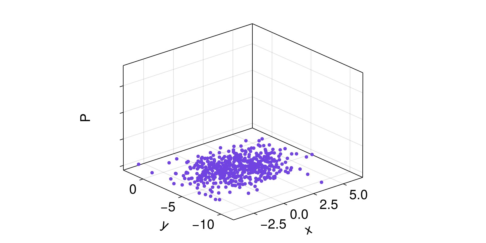

Probabilities: KL-divergence of histograms

In this example we show how simple it is to compute the KL-divergence (or any other distance function for probability distributions) using ComplexityMeasures.jl. For simplicity, we will compute the KL-divergence between the ValueBinnings of two timeseries.

Note that it is crucial to use allprobabilities_and_outcomes instead of probabilities_and_outcomes.

using ComplexityMeasures

N = 1000
t = range(0, 20π; length=N)
x = @. clamp(sin(t), -0.5, 1)
y = @. sin(t + cos(2t))

r = -1:0.1:1
est = ValueBinning(FixedRectangularBinning(r))
px, outsx = allprobabilities_and_outcomes(est, x)
py, outsy = allprobabilities_and_outcomes(est, y)

# Visualize
using CairoMakie
bins = r[1:end-1] .+ step(r)/2
fig, ax = barplot(bins, px; label = L"p_x")
barplot!(ax, bins, py; label = L"p_y")
axislegend(ax; labelsize = 30)
fig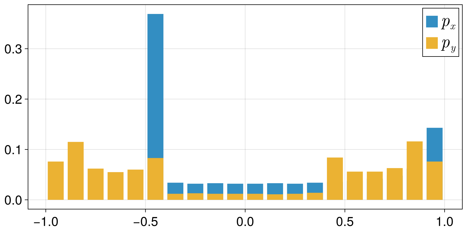

using StatsBase: kldivergence

kldivergence(px, py)

0.7899097070515434

kldivergence(py, px)

Inf

(Inf because there are events with 0 probability in px)

Differential entropy: estimator comparison

Shannon entropy

Here, we compare how the nearest neighbor differential entropy estimators (Kraskov, KozachenkoLeonenko, Zhu, ZhuSingh, etc.) converge towards the true Shannon entropy value for increasing time series length.

ComplexityMeasures.jl also provides entropy estimators based on order statistics. These estimators are only defined for scalar-valued vectors, in this example, so we compute these estimates separately, and add these estimators (Vasicek, Ebrahimi, AlizadehArghami and Correa) to the comparison.

Input data are from a normal 1D distribution $\mathcal{N}(0, 1)$, for which the true entropy is 0.5*log(2π) + 0.5 nats when using natural logarithms.

using ComplexityMeasures
using CairoMakie, Statistics
nreps = 30
Ns = [100:100:500; 1000:1000:5000]
e = Shannon(; base = MathConstants.e)

# --------------------------
# kNN estimators
# --------------------------
w = 0 # Theiler window of 0 (only exclude the point itself during neighbor searches)
ent = Shannon(; base = ℯ)
knn_estimators = [
    # with k = 1, Kraskov is virtually identical to
    # Kozachenko-Leonenko, so pick a higher number of neighbors for Kraskov
    Kraskov(ent; k = 3, w),
    KozachenkoLeonenko(ent; w),
    Zhu(ent; k = 3, w),
    ZhuSingh(ent; k = 3, w),
    Gao(ent; k = 3, corrected = false, w),
    Gao(ent; k = 3, corrected = true, w),
    Goria(ent; k = 3, w),
    Lord(ent; k = 20, w), # more neighbors for accurate ellipsoid estimation
    LeonenkoProzantoSavani(ent; k = 3),
]

# Test each estimator `nreps` times over time series of varying length.
Hs_uniform_knn = [[zeros(nreps) for N in Ns] for e in knn_estimators]
for (i, est) in enumerate(knn_estimators)
    for j = 1:nreps
        pts = randn(maximum(Ns)) |> StateSpaceSet
        for (k, N) in enumerate(Ns)
            Hs_uniform_knn[i][k][j] = information(est, pts[1:N])
        end
    end
end

# --------------------------
# Order statistic estimators
# --------------------------

# Just provide types here, they are instantiated inside the loop
estimators_os = [Vasicek, Ebrahimi, AlizadehArghami, Correa]
Hs_uniform_os = [[zeros(nreps) for N in Ns] for e in estimators_os]
for (i, est_os) in enumerate(estimators_os)
    for j = 1:nreps
        pts = randn(maximum(Ns)) # raw timeseries, not a `StateSpaceSet`
        for (k, N) in enumerate(Ns)
            m = floor(Int, N / 100) # Scale `m` to timeseries length
            est = est_os(ent; m) # Instantiate estimator with current `m`
            Hs_uniform_os[i][k][j] = information(est, pts[1:N])
        end
    end
end

# -------------
# Plot results
# -------------
fig = Figure(resolution = (700, 11 * 200))
labels_knn = ["KozachenkoLeonenko", "Kraskov", "Zhu", "ZhuSingh", "Gao (not corrected)",
    "Gao (corrected)", "Goria", "Lord", "LeonenkoProzantoSavani"]
labels_os = ["Vasicek", "Ebrahimi", "AlizadehArghami", "Correa"]

for (i, e) in enumerate(knn_estimators)
    Hs = Hs_uniform_knn[i]
    ax = Axis(fig[i,1]; ylabel = "h (nats)")
    lines!(ax, Ns, mean.(Hs); color = Cycled(i), label = labels_knn[i])
    band!(ax, Ns, mean.(Hs) .+ std.(Hs), mean.(Hs) .- std.(Hs); alpha = 0.5,
        color = (Main.COLORS[i], 0.5))
    hlines!(ax, [(0.5*log(2π) + 0.5)], color = :black, linewidth = 5, linestyle = :dash)

    ylims!(1.2, 1.6)
    axislegend()
end

for (i, e) in enumerate(estimators_os)
    Hs = Hs_uniform_os[i]
    ax = Axis(fig[i + length(knn_estimators),1]; ylabel = "h (nats)")
    lines!(ax, Ns, mean.(Hs); color = Cycled(i), label = labels_os[i])
    band!(ax, Ns, mean.(Hs) .+ std.(Hs), mean.(Hs) .- std.(Hs), alpha = 0.5,
        color = (Main.COLORS[i], 0.5))
    hlines!(ax, [(0.5*log(2π) + 0.5)], color = :black, linewidth = 5, linestyle = :dash)
    ylims!(1.2, 1.6)
    axislegend()
end

fig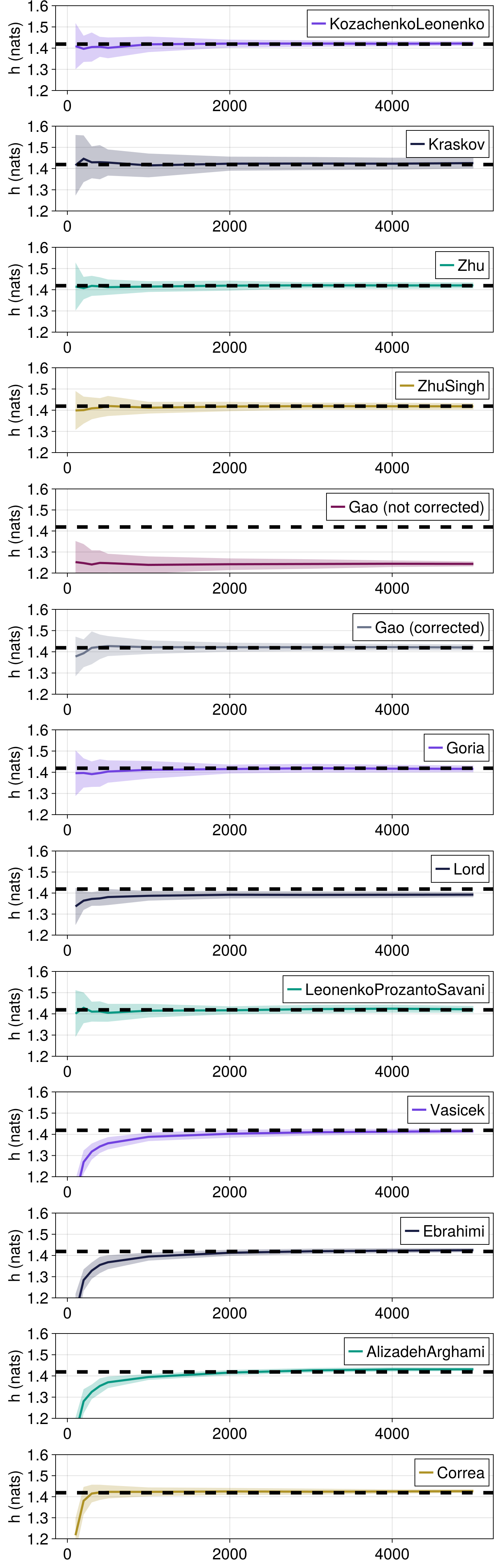

All estimators approach the true differential entropy, but those based on order statistics are negatively biased for small sample sizes.

Rényi entropy

Here, we see how the LeonenkoProzantoSavani estimator approaches the known target Renyi entropy of a multivariate normal distribution for increasing time series length. We'll consider the Rényi entropy with q = 2.

using ComplexityMeasures
import ComplexityMeasures: information # we're overriding this function in the example
using CairoMakie, Statistics
using Distributions: MvNormal
import Distributions.entropy as dentropy
using Random
rng = MersenneTwister(1234)

"""
    information(e::Renyi, 𝒩::MvNormal; base = 2)

Compute the analytical value of the `Renyi` entropy for a multivariate normal distribution.
"""
function information(e::Renyi, 𝒩::MvNormal; base = 2)
    q = e.q
    if q ≈ 1.0
        h = dentropy(𝒩)
    else
        Σ = 𝒩.Σ
        D = length(𝒩.μ)
        h = dentropy(𝒩) - (D / 2) * (1 + log(q) / (1 - q))
    end
    return convert_logunit(h, ℯ, base)
end

nreps = 30
Ns = [100:100:500; 1000:1000:5000]
def = Renyi(q = 2, base = 2)

μ = [-1, 1]
σ = [1, 0.5]
𝒩 = MvNormal(μ, LinearAlgebra.Diagonal(map(abs2, σ)))
h_true = information(def, 𝒩; base = 2)

# Estimate `nreps` times for each time series length

hs = [zeros(nreps) for N in Ns]
for (i, N) in enumerate(Ns)
    for j = 1:nreps
        pts = StateSpaceSet(transpose(rand(rng, 𝒩, N)))
        hs[i][j] = information(LeonenkoProzantoSavani(def; k = 5), pts)
    end
end

# We plot the mean and standard deviation of the estimator again the true value
hs_mean, hs_stdev = mean.(hs), std.(hs)

fig = Figure()
ax = Axis(fig[1, 1]; ylabel = "h (bits)")
lines!(ax, Ns, hs_mean; color = Cycled(1), label = "LeonenkoProzantoSavani")
band!(ax, Ns, hs_mean .+ hs_stdev, hs_mean .- hs_stdev,
    alpha = 0.5, color = (Main.COLORS[1], 0.5))
hlines!(ax, [h_true], color = :black, linewidth = 5, linestyle = :dash)
axislegend()
fig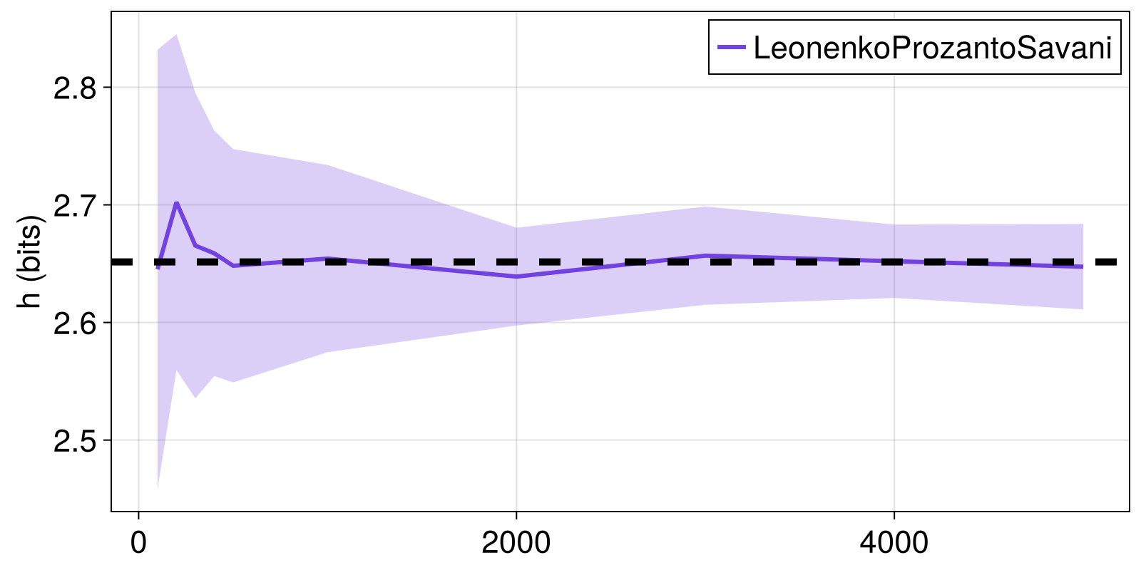

Tsallis entropy

Here, we see how the LeonenkoProzantoSavani estimator approaches the known target Tsallis entropy of a multivariate normal distribution for increasing time series length. We'll consider the Rényi entropy with q = 2.

using ComplexityMeasures
import ComplexityMeasures: information # we're overriding this function in the example
using CairoMakie, Statistics
using Distributions: MvNormal
import Distributions.entropy as dentropy
using Random
rng = MersenneTwister(1234)

"""
    information(e::Tsallis, 𝒩::MvNormal; base = 2)

Compute the analytical value of the `Tsallis` entropy for a multivariate normal distribution.
"""
function information(e::Tsallis, 𝒩::MvNormal; base = 2)
    q = e.q
    Σ = 𝒩.Σ
    D = length(𝒩.μ)
    # uses the function from the example above
    hr = information(Renyi(q = q), 𝒩; base = ℯ) # stick with natural log, convert after
    h = (exp((1 - q) * hr) - 1) / (1 - q)
    return convert_logunit(h, ℯ, base)
end

nreps = 30
Ns = [100:100:500; 1000:1000:5000]
def = Tsallis(q = 2, base = 2)

μ = [-1, 1]
σ = [1, 0.5]
𝒩 = MvNormal(μ, LinearAlgebra.Diagonal(map(abs2, σ)))
h_true = information(def, 𝒩; base = 2)

# Estimate `nreps` times for each time series length

hs = [zeros(nreps) for N in Ns]
for (i, N) in enumerate(Ns)
    for j = 1:nreps
        pts = StateSpaceSet(transpose(rand(rng, 𝒩, N)))
        hs[i][j] = information(LeonenkoProzantoSavani(def; k = 5), pts)
    end
end

# We plot the mean and standard deviation of the estimator again the true value
hs_mean, hs_stdev = mean.(hs), std.(hs)

fig = Figure()
ax = Axis(fig[1, 1]; ylabel = "h (bits)")
lines!(ax, Ns, hs_mean; color = Cycled(1), label = "LeonenkoProzantoSavani")
band!(ax, Ns, hs_mean .+ hs_stdev, hs_mean .- hs_stdev,
    alpha = 0.5, color = (Main.COLORS[1], 0.5))
hlines!(ax, [h_true], color = :black, linewidth = 5, linestyle = :dash)
axislegend()
fig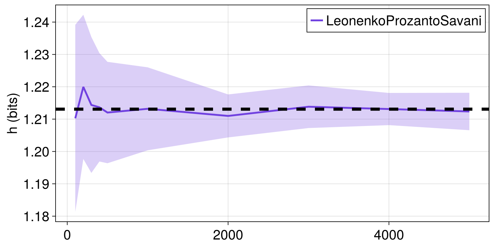

Discrete entropy: permutation entropy

This example plots permutation entropy for time series of the chaotic logistic map. Entropy estimates using WeightedOrdinalPatterns and AmplitudeAwareOrdinalPatterns are added here for comparison. The entropy behaviour can be parallelized with the ChaosTools.lyapunov of the map.

using DynamicalSystemsBase, CairoMakie

logistic_rule(x, p, n) = @inbounds SVector(p[1]*x[1]*(1-x[1]))
ds = DeterministicIteratedMap(logistic_rule, [0.4], [4.0])
rs = 3.4:0.001:4
N_lyap, N_ent = 100000, 10000
m, τ = 6, 1 # Symbol size/dimension and embedding lag

# Generate one time series for each value of the logistic parameter r
hs_perm, hs_wtperm, hs_ampperm = [zeros(length(rs)) for _ in 1:4]

for (i, r) in enumerate(rs)
    ds.p[1] = r

    x, t = trajectory(ds, N_ent)
    ## `x` is a 1D dataset, need to recast into a timeseries
    x = columns(x)[1]
    hs_perm[i] = information(OrdinalPatterns(; m, τ), x)
    hs_wtperm[i] = information(WeightedOrdinalPatterns(; m, τ), x)
    hs_ampperm[i] = information(AmplitudeAwareOrdinalPatterns(; m, τ), x)
end

fig = Figure()
a1 = Axis(fig[1,1]; ylabel = L"h_6 (SP)")
lines!(a1, rs, hs_perm; color = Cycled(2))
a2 = Axis(fig[2,1]; ylabel = L"h_6 (WT)")
lines!(a2, rs, hs_wtperm; color = Cycled(3))
a3 = Axis(fig[3,1]; ylabel = L"h_6 (SAAP)", xlabel = L"r")
lines!(a3, rs, hs_ampperm; color = Cycled(4))

for a in (a1,a2,a3)
    hidexdecorations!(a, grid = false)
end
fig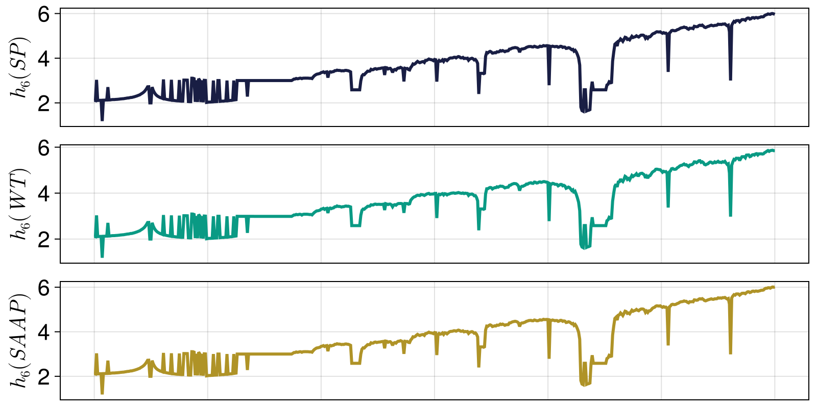

Discrete entropy: wavelet entropy

The scale-resolved wavelet entropy should be lower for very regular signals (most of the energy is contained at one scale) and higher for very irregular signals (energy spread more out across scales).

using CairoMakie
N, a = 1000, 10
t = LinRange(0, 2*a*π, N)

x = sin.(t);
y = sin.(t .+ cos.(t/0.5));
z = sin.(rand(1:15, N) ./ rand(1:10, N))

h_x = entropy_wavelet(x)
h_y = entropy_wavelet(y)
h_z = entropy_wavelet(z)

fig = Figure()
ax = Axis(fig[1,1]; ylabel = "x")
lines!(ax, t, x; color = Cycled(1), label = "h=$(h=round(h_x, sigdigits = 5))");
ay = Axis(fig[2,1]; ylabel = "y")
lines!(ay, t, y; color = Cycled(2), label = "h=$(h=round(h_y, sigdigits = 5))");
az = Axis(fig[3,1]; ylabel = "z", xlabel = "time")
lines!(az, t, z; color = Cycled(3), label = "h=$(h=round(h_z, sigdigits = 5))");
for a in (ax, ay, az); axislegend(a); end
for a in (ax, ay); hidexdecorations!(a; grid=false); end
fig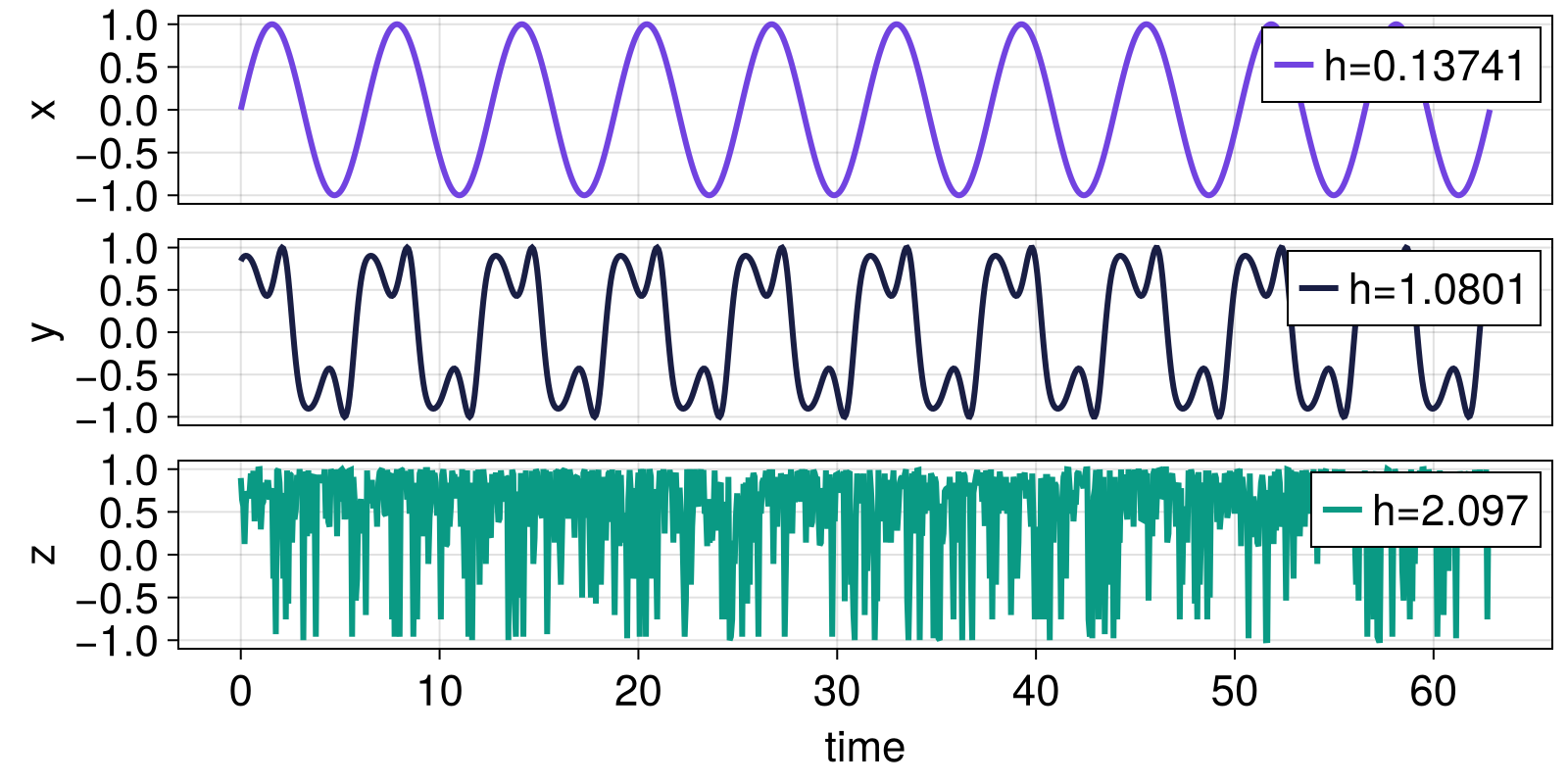

Discrete entropies: properties

Here, we show the sensitivity of the various entropies to variations in their parameters.

Curado entropy

Here, we reproduce Figure 2 from Curado and Nobre (2004), showing how the Curado entropy changes as function of the parameter a for a range of two-element probability distributions given by Probabilities([p, 1 - p] for p in 1:0.0:0.01:1.0).

using ComplexityMeasures, CairoMakie
bs = [1.0, 1.5, 2.0, 3.0, 4.0, 10.0]
ps = [Probabilities([p, 1 - p]) for p = 0.0:0.01:1.0]
hs = [[information(Curado(; b = b), p) for p in ps] for b in bs]
fig = Figure()
ax = Axis(fig[1,1]; xlabel = "p", ylabel = "H(p)")
pp = [p[1] for p in ps]
for (i, b) in enumerate(bs)
    lines!(ax, pp, hs[i], label = "b=$b", color = Cycled(i))
end
axislegend(ax)
fig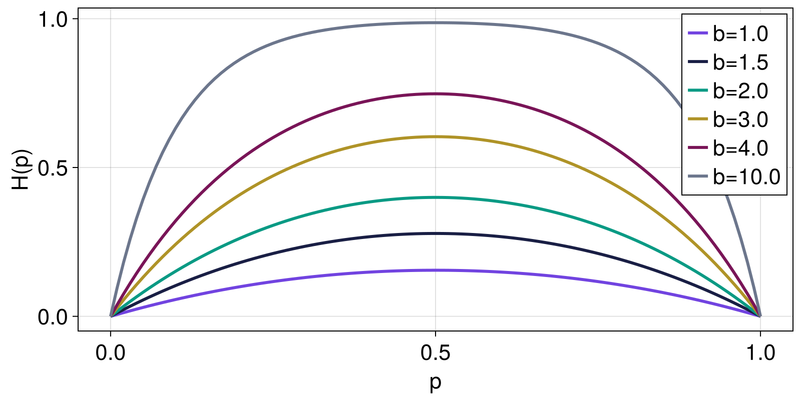

Kaniadakis entropy

Here, we show how Kaniadakis entropy changes as function of the parameter a for a range of two-element probability distributions given by Probabilities([p, 1 - p] for p in 1:0.0:0.01:1.0).

using ComplexityMeasures
using CairoMakie

probs = [Probabilities([p, 1-p]) for p in 0.0:0.01:1.0]
ps = collect(0.0:0.01:1.0);
κs = [-0.99, -0.66, -0.33, 0, 0.33, 0.66, 0.99];
Hs = [[information(Kaniadakis(κ = κ), p) for p in probs] for κ in κs];

fig = Figure()
ax = Axis(fig[1, 1], xlabel = "p", ylabel = "H(p)")

for (i, H) in enumerate(Hs)
    lines!(ax, ps, H, label = "$(κs[i])")
end

axislegend()

fig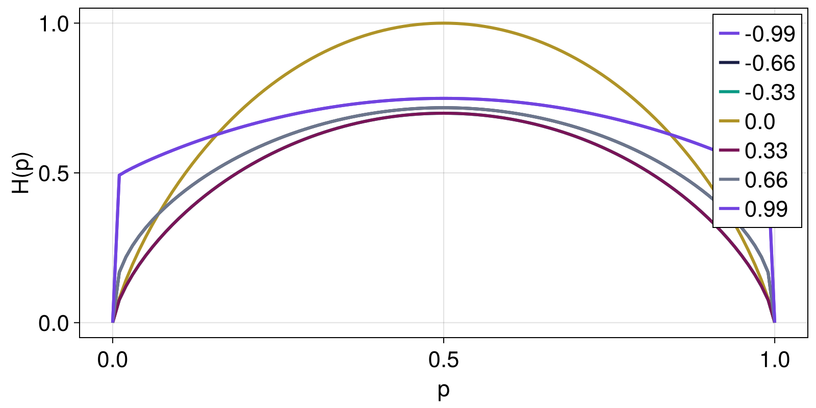

Stretched exponential entropy

Here, we reproduce the example from Anteneodo and Plastino (1999), showing how the stretched exponential entropy changes as function of the parameter η for a range of two-element probability distributions given by Probabilities([p, 1 - p] for p in 1:0.0:0.01:1.0).

using ComplexityMeasures, SpecialFunctions, CairoMakie
ηs = [0.01, 0.2, 0.3, 0.5, 0.7, 1.0, 1.5, 3.0]
ps = [Probabilities([p, 1 - p]) for p = 0.0:0.01:1.0]

hs_norm = [[information(StretchedExponential( η = η), p) / gamma((η + 1)/η) for p in ps] for η in ηs]
fig = Figure()
ax = Axis(fig[1,1]; xlabel = "p", ylabel = "H(p)")
pp = [p[1] for p in ps]

for (i, η) in enumerate(ηs)
    lines!(ax, pp, hs_norm[i], label = "η=$η")
end
axislegend(ax)
fig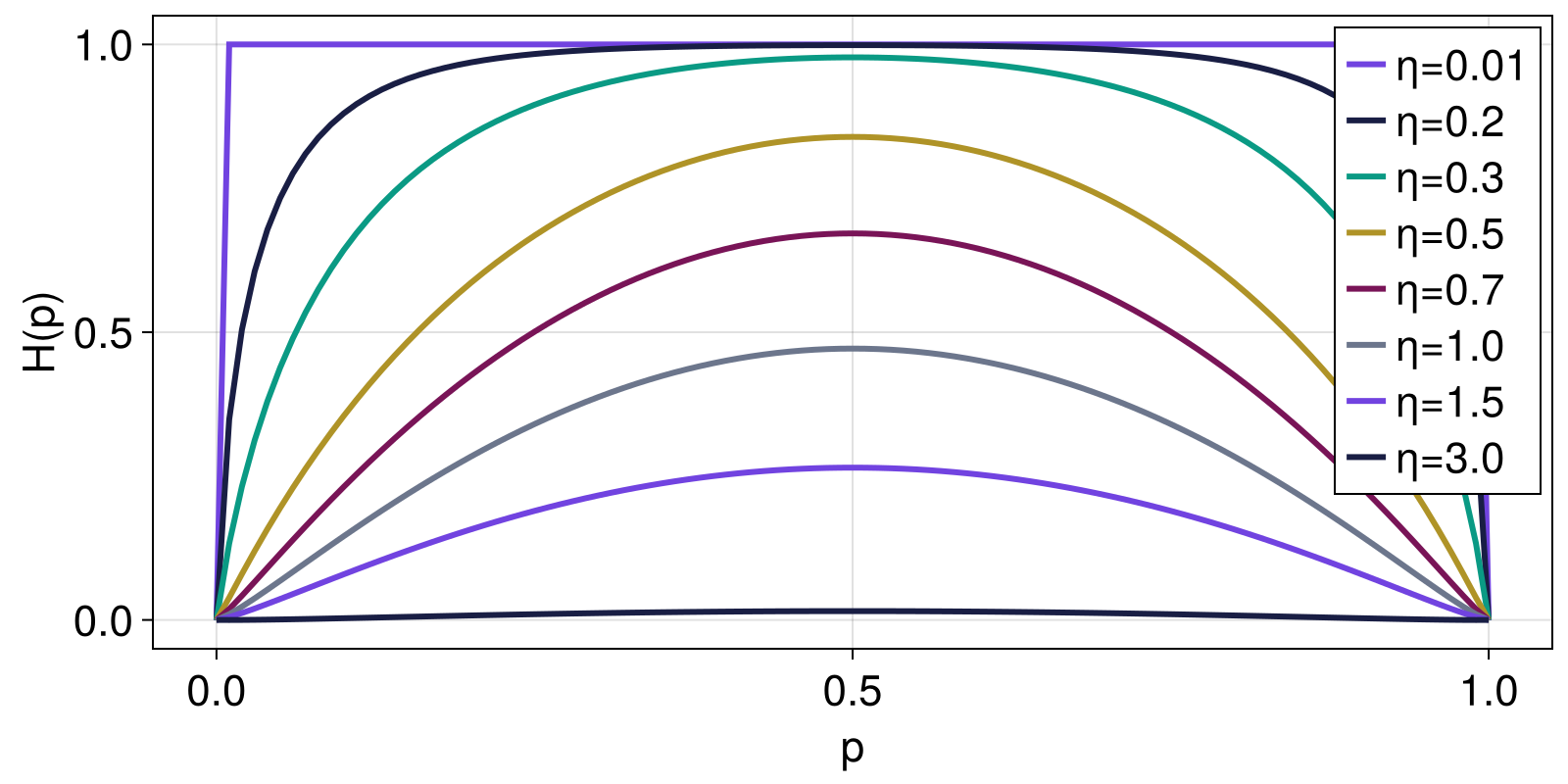

Discrete entropy: dispersion entropy

Here we compute dispersion entropy (Rostaghi and Azami, 2016), using the use the Dispersion probabilities estimator, for a time series consisting of normally distributed noise with a single spike in the middle of the signal. We compute the entropies over a range subsets of the data, using a sliding window consisting of 70 data points, stepping the window 10 time steps at a time. This example is adapted from Li et al. (2019).

using ComplexityMeasures
using Random
using CairoMakie
using Distributions: Normal

n = 1000
ts = 1:n
x = [i == n ÷ 2 ? 50.0 : 0.0 for i in ts]
rng = Random.default_rng()
s = rand(rng, Normal(0, 1), n)
y = x .+ s

ws = 70
windows = [t:t+ws for t in 1:10:n-ws]
rdes = zeros(length(windows))
des = zeros(length(windows))
pes = zeros(length(windows))

m, c = 2, 6
est_de = Dispersion(c = c, m = m, τ = 1)
for (i, window) in enumerate(windows)
    des[i] = information_normalized(Renyi(), est_de, y[window])
end

fig = Figure()
a1 = Axis(fig[1,1]; xlabel = "Time step", ylabel = "Value")
lines!(a1, ts, y)
display(fig)
a2 = Axis(fig[2, 1]; xlabel = "Time step", ylabel = "Value")
p_de = scatterlines!([first(w) for w in windows], des,
    label = "Dispersion entropy",
    color = :red,
    markercolor = :red, marker = '●', markersize = 20)

axislegend(position = :rc)
ylims!(0, max(maximum(pes), 1))
fig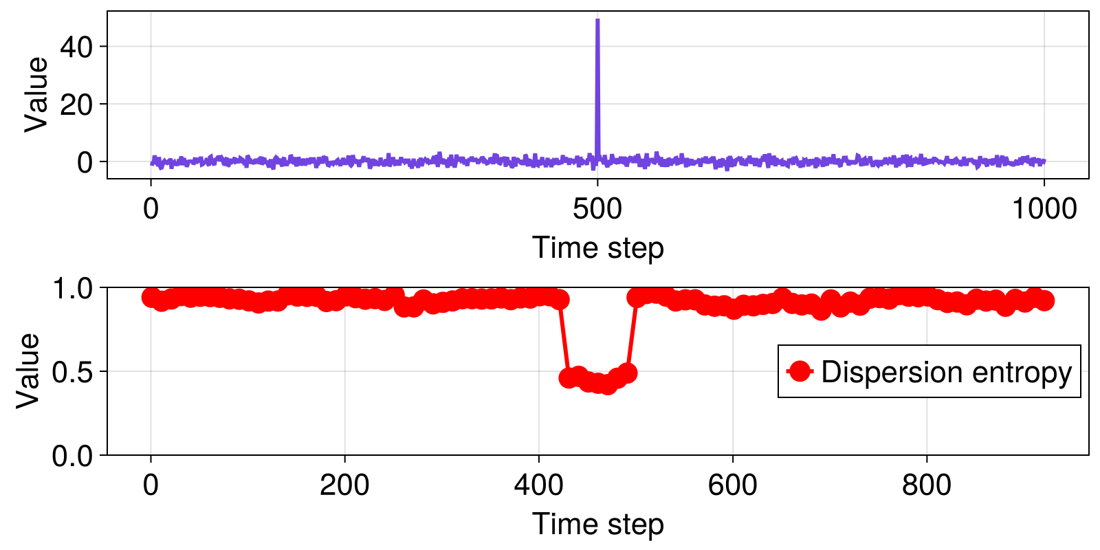

Discrete entropy: normalized entropy for comparing different signals

When comparing different signals or signals that have different length, it is best to normalize entropies so that the "complexity" or "disorder" quantification is directly comparable between signals. Here is an example based on the wavelet entropy example where we use the spectral entropy instead of the wavelet entropy:

using ComplexityMeasures
N1, N2, a = 101, 10001, 10

for N in (N1, N2)
    local t = LinRange(0, 2*a*π, N)
    local x = sin.(t) # periodic
    local y = sin.(t .+ cos.(t/0.5)) # periodic, complex spectrum
    local z = sin.(rand(1:15, N) ./ rand(1:10, N)) # random

    for q in (x, y, z)
        local h = information(PowerSpectrum(), q)
        local n = information_normalized(PowerSpectrum(), q)
        println("entropy: $(h), normalized: $(n).")
    end
end

entropy: 0.3131510976800182, normalized: 0.05520585619046334.
entropy: 1.2651873361559447, normalized: 0.22304169026158024.
entropy: 2.851432844069554, normalized: 0.5026831861445913.
entropy: 7.57800737722389e-5, normalized: 6.1669977445812415e-6.
entropy: 0.8397257036159657, normalized: 0.06833704775520644.
entropy: 5.3146902488941965, normalized: 0.4325105683663955.

You see that while the direct entropy values of noisy signal changes strongly with N but they are almost the same for the normalized version. For the regular signals, the entropy decreases nevertheless because the noise contribution of the Fourier computation becomes less significant.

Spatiotemporal permutation entropy

Usage of a SpatialOrdinalPatterns estimator is straightforward. Here we get the spatial permutation entropy of a 2D array (e.g., an image):

using ComplexityMeasures
x = rand(50, 50) # some image
stencil = [1 1; 0 1] # or one of the other ways of specifying stencils
est = SpatialOrdinalPatterns(stencil, x)
h = information(est, x)

2.584080549086423

To apply this to timeseries of spatial data, simply loop over the call, e.g.:

data = [rand(50, 50) for i in 1:10] # e.g., evolution of a 2D field of a PDE
est = SpatialOrdinalPatterns(stencil, first(data))
h_vs_t = map(d -> information(est, d), data)

10-element Vector{Float64}:
 2.584601037992588
 2.584546536964212
 2.5834277316350027
 2.584453704567631
 2.5839792525715484
 2.5829861828434324
 2.5846710919495193
 2.584688394079985
 2.583965225840613
 2.583557083067056

Computing any other generalized spatiotemporal permutation entropy is trivial, e.g. with Renyi:

x = reshape(repeat(1:5, 500) .+ 0.1*rand(500*5), 50, 50)
est = SpatialOrdinalPatterns(stencil, x)
information(Renyi(q = 2), est, x)

1.5563064499814285

Spatial discrete entropy: Fabio

Let's see how the normalized permutation and dispersion entropies increase for an image that gets progressively more noise added to it.

using ComplexityMeasures
using Distributions: Uniform
using CairoMakie
using Statistics
using TestImages, ImageTransformations, CoordinateTransformations, Rotations

img = testimage("fabio_grey_256")
rot = warp(img, recenter(RotMatrix(-3pi/2), center(img));)
original = Float32.(rot)
noise_levels = collect(0.0:0.25:1.0) .* std(original) * 5 # % of 1 standard deviation

noisy_imgs = [i == 1 ? original : original .+ rand(Uniform(0, nL), size(original))
    for (i, nL) in enumerate(noise_levels)]

# a 2x2 stencil (i.e. dispersion/permutation patterns of length 4)
stencil = ((2, 2), (1, 1))

est_disp = SpatialDispersion(stencil, original; c = 5, periodic = false)
est_perm = SpatialOrdinalPatterns(stencil, original; periodic = false)
hs_disp = [information_normalized(est_disp, img) for img in noisy_imgs]
hs_perm = [information_normalized(est_perm, img) for img in noisy_imgs]

# Plot the results
fig = Figure(size = (800, 1000))
ax = Axis(fig[1, 1:length(noise_levels)],
    xlabel = "Noise level",
    ylabel = "Normalized entropy")
scatterlines!(ax, noise_levels, hs_disp, label = "Dispersion")
scatterlines!(ax, noise_levels, hs_perm, label = "Permutation")
ylims!(ax, 0, 1.05)
axislegend(position = :rb)
for (i, nl) in enumerate(noise_levels)
    ax_i = Axis(fig[2, i])
    image!(ax_i, Matrix(Float32.(noisy_imgs[i])), label = "$nl")
    hidedecorations!(ax_i)  # hides ticks, grid and lables
    hidespines!(ax_i)  # hide the frame
end
fig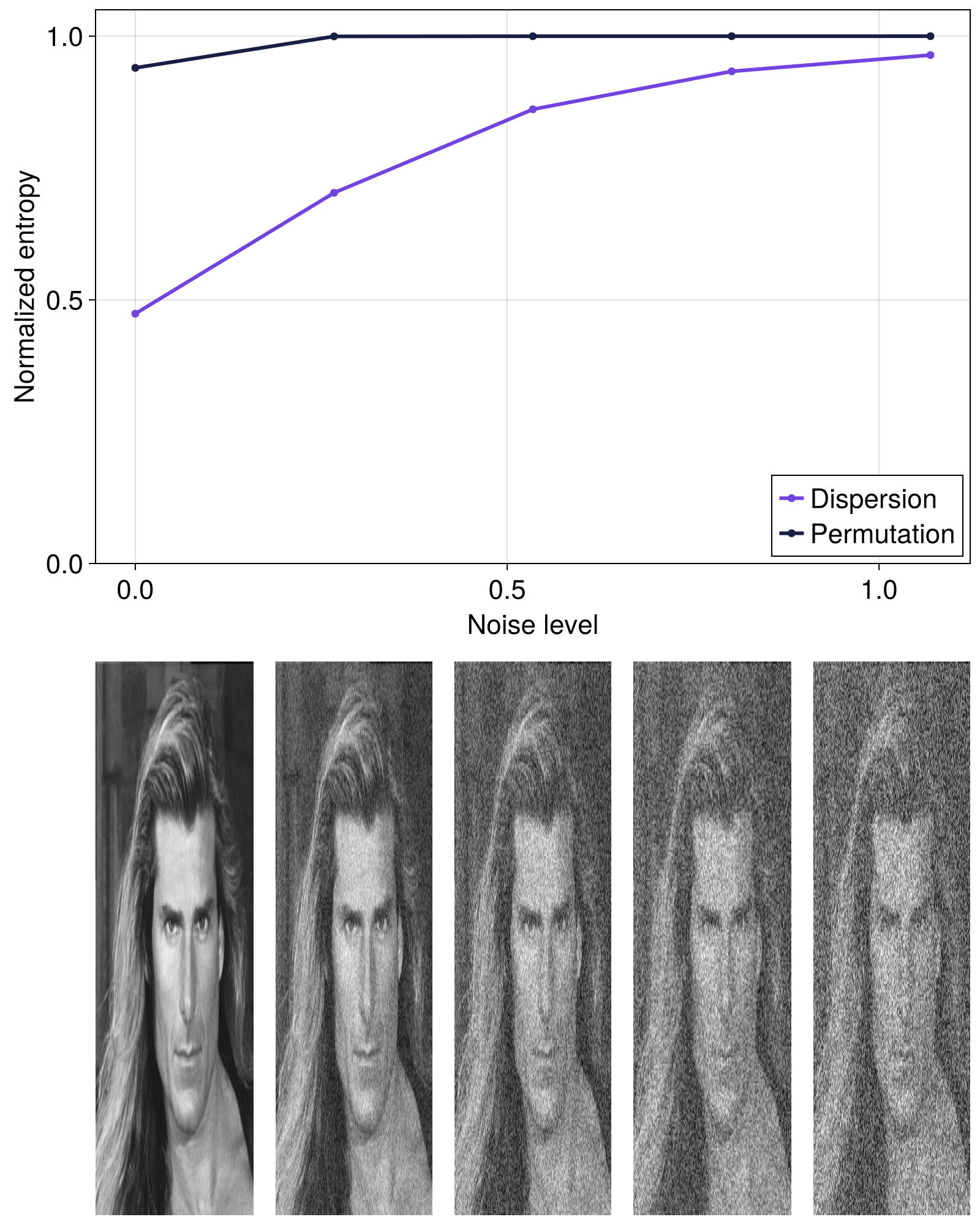

While the normalized SpatialOrdinalPatterns entropy quickly approaches its maximum value, the normalized SpatialDispersion entropy much better resolves the increase in entropy as the image gets noiser. This can probably be explained by the fact that the number of possible states (or total_outcomes) for any given stencil is larger for SpatialDispersion than for SpatialOrdinalPatterns, so the dispersion approach is much less sensitive to noise addition (i.e. noise saturation over the possible states is slower for SpatialDispersion).

Complexity: reverse dispersion entropy

Here, we compare regular dispersion entropy (Rostaghi and Azami, 2016), and reverse dispersion entropy (Li et al., 2019) for a time series consisting of normally distributed noise with a single spike in the middle of the signal. We compute the entropies over a range subsets of the data, using a sliding window consisting of 70 data points, stepping the window 10 time steps at a time. This example reproduces parts of figure 3 in (Li et al., 2019), but results here are not exactly the same as in the original paper, because their examples are based on randomly generated numbers and do not provide code that specify random number seeds.

using ComplexityMeasures
using Random
using CairoMakie
using Distributions: Normal

n = 1000
ts = 1:n
x = [i == n ÷ 2 ? 50.0 : 0.0 for i in ts]
rng = Random.default_rng()
s = rand(rng, Normal(0, 1), n)
y = x .+ s

ws = 70
windows = [t:t+ws for t in 1:10:n-ws]
rdes = zeros(length(windows))
des = zeros(length(windows))
pes = zeros(length(windows))

m, c = 2, 6
est_rd = ReverseDispersion(; c, m, τ = 1)
est_de = Dispersion(; c, m, τ = 1)

for (i, window) in enumerate(windows)
    rdes[i] = complexity_normalized(est_rd, y[window])
    des[i] = information_normalized(Renyi(), est_de, y[window])
end

fig = Figure()

a1 = Axis(fig[1,1]; xlabel = "Time step", ylabel = "Value")
lines!(a1, ts, y)
display(fig)

a2 = Axis(fig[2, 1]; xlabel = "Time step", ylabel = "Value")
p_rde = scatterlines!([first(w) for w in windows], rdes,
    label = "Reverse dispersion entropy",
    color = :black,
    markercolor = :black, marker = '●')
p_de = scatterlines!([first(w) for w in windows], des,
    label = "Dispersion entropy",
    color = :red,
    markercolor = :red, marker = 'x', markersize = 20)

axislegend(position = :rc)
ylims!(0, max(maximum(pes), 1))
fig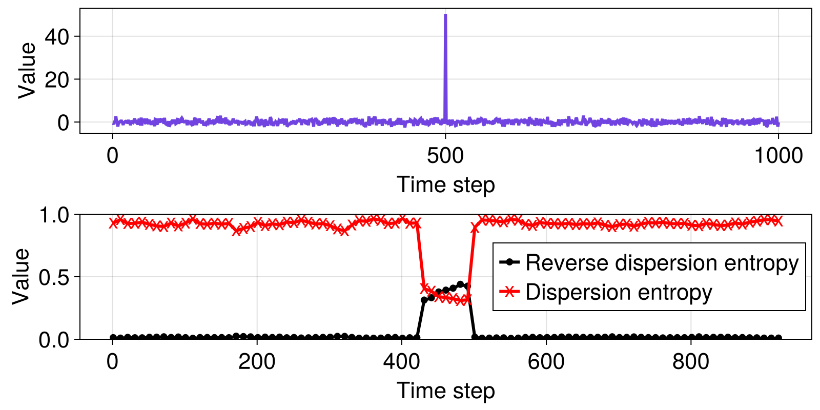

Complexity: missing dispersion patterns

using ComplexityMeasures
using CairoMakie
using DynamicalSystemsBase
using TimeseriesSurrogates

est = MissingDispersionPatterns(Dispersion(m = 3, c = 7))
logistic_rule(x, p, n) = @inbounds SVector(p[1]*x[1]*(1-x[1]))
sys = DeterministicIteratedMap(logistic_rule, [0.6], [4.0])
Ls = collect(100:100:1000)
nL = length(Ls)
nreps = 30 # should be higher for real applications
method = WLS(IAAFT(), rescale = true)

r_det, r_noise = zeros(length(Ls)), zeros(length(Ls))
r_det_surr, r_noise_surr = [zeros(nreps) for L in Ls], [zeros(nreps) for L in Ls]
y = rand(maximum(Ls))

for (i, L) in enumerate(Ls)
    # Deterministic time series
    x, t = trajectory(sys, L - 1, Ttr = 5000)
    x = columns(x)[1] # remember to make it `Vector{<:Real}
    sx = surrogenerator(x, method)
    r_det[i] = complexity_normalized(est, x)
    r_det_surr[i][:] = [complexity_normalized(est, sx()) for j = 1:nreps]

    # Random time series
    r_noise[i] = complexity_normalized(est, y[1:L])
    sy = surrogenerator(y[1:L], method)
    r_noise_surr[i][:] = [complexity_normalized(est, sy()) for j = 1:nreps]
end

fig = Figure()
ax = Axis(fig[1, 1],
    xlabel = "Time series length (L)",
    ylabel = "# missing dispersion patterns (normalized)"
)

lines!(ax, Ls, r_det, label = "logistic(x0 = 0.6; r = 4.0)", color = :black)
lines!(ax, Ls, r_noise, label = "Uniform noise", color = :red)
for i = 1:nL
    if i == 1
        boxplot!(ax, fill(Ls[i], nL), r_det_surr[i]; width = 50, color = :black,
            label = "WIAAFT surrogates (logistic)")
         boxplot!(ax, fill(Ls[i], nL), r_noise_surr[i]; width = 50, color = :red,
            label = "WIAAFT surrogates (noise)")
    else
        boxplot!(ax, fill(Ls[i], nL), r_det_surr[i]; width = 50, color = :black)
        boxplot!(ax, fill(Ls[i], nL), r_noise_surr[i]; width = 50, color = :red)
    end
end
axislegend(position = :rc)
ylims!(0, 1.1)

fig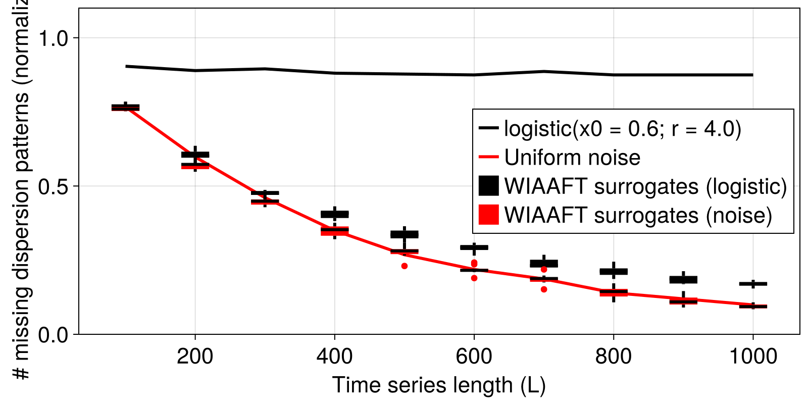

We don't need to actually to compute the quantiles here to see that for the logistic map, across all time series lengths, the $N_{MDP}$ values are above the extremal values of the $N_{MDP}$ values for the surrogate ensembles. Thus, we conclude that the logistic map time series has nonlinearity (well, of course).

For the univariate noise time series, there is considerable overlap between $N_{MDP}$ for the surrogate distributions and the original signal, so we can't claim nonlinearity for this signal.

Of course, to robustly reject the null hypothesis, we'd need to generate a sufficient number of surrogate realizations, and actually compute quantiles to compare with.

Complexity: approximate entropy

Here, we reproduce the Henon map example with $R=0.8$ from Pincus (1991), comparing our values with relevant values from table 1 in Pincus (1991).

We use DiscreteDynamicalSystem from DynamicalSystemsBase to represent the map, and use the trajectory function from the same package to iterate the map for different initial conditions, for multiple time series lengths.

Finally, we summarize our results in box plots and compare the values to those obtained by Pincus (1991).

using ComplexityMeasures
using DynamicalSystemsBase
using DelayEmbeddings
using CairoMakie

# Equation 13 in Pincus (1991)
function henon_rule(u, p, n)
    R = p[1]
    x, y = u
    dx = R*y + 1 - 1.4*x^2
    dy = 0.3*R*x
    return SVector(dx, dy)
end

function henon(; u₀ = rand(2), R = 0.8)
    DeterministicIteratedMap(henon_rule, u₀, [R])
end

ts_lengths = [300, 1000, 2000, 3000]
nreps = 100
apens_08 = [zeros(nreps) for i = 1:length(ts_lengths)]

# For some initial conditions, the Henon map as specified here blows up,
# so we need to check for infinite values.
containsinf(x) = any(isinf.(x))

c = ApproximateEntropy(r = 0.05, m = 2)

for (i, L) in enumerate(ts_lengths)
    k = 1
    while k <= nreps
        sys = henon(u₀ = rand(2), R = 0.8)
        t = trajectory(sys, L; Ttr = 5000)[1]

        if !any([containsinf(tᵢ) for tᵢ in t])
            x, y = columns(t)
            apens_08[i][k] = complexity(c, x)
            k += 1
        end
    end
end

fig = Figure()

# Example time series
a1 = Axis(fig[1,1]; xlabel = "Time (t)", ylabel = "Value")
sys = henon(u₀ = [0.5, 0.1], R = 0.8)
x, y = columns(first(trajectory(sys, 100, Ttr = 500))) # we don't need time indices
lines!(a1, 1:length(x), x, label = "x")
lines!(a1, 1:length(y), y, label = "y")

# Approximate entropy values, compared to those of the original paper (black dots).
a2 = Axis(fig[2, 1];
    xlabel = "Time series length (L)",
    ylabel = "ApEn(m = 2, r = 0.05)")

# hacky boxplot, but this seems to be how it's done in Makie at the moment
n = length(ts_lengths)
for i = 1:n
    boxplot!(a2, fill(ts_lengths[i], n), apens_08[i];
        width = 200)
end

scatter!(a2, ts_lengths, [0.337, 0.385, NaN, 0.394];
    label = "Pincus (1991)", color = :black)
fig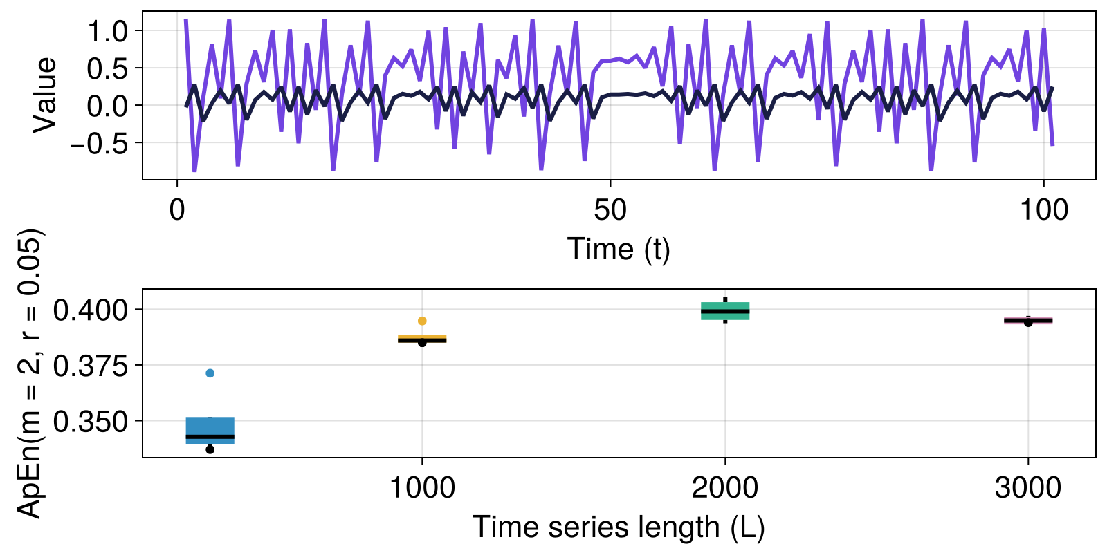

Complexity: sample entropy

Completely regular signals should have sample entropy approaching zero, while less regular signals should have higher sample entropy.

using ComplexityMeasures
using CairoMakie
N, a = 2000, 10
t = LinRange(0, 2*a*π, N)

x = repeat([-5:5.0 |> collect; 4.0:-1:-4 |> collect], N ÷ 20);
y = sin.(t .+ cos.(t/0.5));
z = rand(N)

h_x, h_y, h_z = map(t -> complexity(SampleEntropy(t), t), (x, y, z))

fig = Figure()
ax = Axis(fig[1,1]; ylabel = "x")
lines!(ax, t, x; color = Cycled(1), label = "h=$(h=round(h_x, sigdigits = 5))");
ay = Axis(fig[2,1]; ylabel = "y")
lines!(ay, t, y; color = Cycled(2), label = "h=$(h=round(h_y, sigdigits = 5))");
az = Axis(fig[3,1]; ylabel = "z", xlabel = "time")
lines!(az, t, z; color = Cycled(3), label = "h=$(h=round(h_z, sigdigits = 5))");
for a in (ax, ay, az); axislegend(a); end
for a in (ax, ay); hidexdecorations!(a; grid=false); end
fig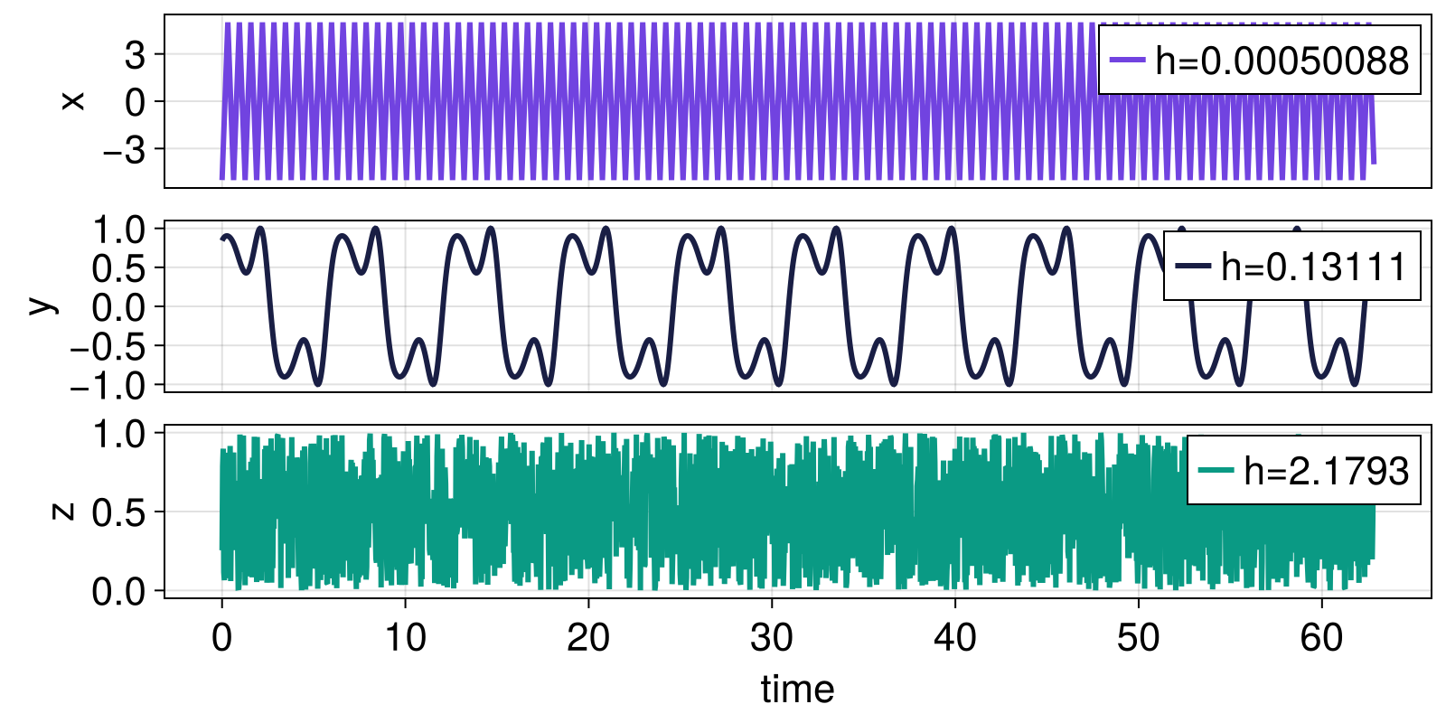

Next, we compare the sample entropy obtained for different values of the radius r for uniform noise, normally distributed noise, and a periodic signal.

using ComplexityMeasures
using CairoMakie
using Statistics
using Distributions: Normal
N = 2000
x_U = rand(N)
x_N = rand(Normal(0, 3), N)
x_periodic = repeat(rand(20), N ÷ 20)

x_U .= (x_U .- mean(x_U)) ./ std(x_U)
x_N .= (x_N .- mean(x_N)) ./ std(x_N)
x_periodic .= (x_periodic .- mean(x_periodic)) ./ std(x_periodic)

rs = 10 .^ range(-1, 0, length = 30)
base = 2
m = 2
hs_U = [complexity_normalized(SampleEntropy(m = m, r = r), x_U) for r in rs]
hs_N = [complexity_normalized(SampleEntropy(m = m, r = r), x_N) for r in rs]
hs_periodic = [complexity_normalized(SampleEntropy(m = m, r = r), x_periodic) for r in rs]

fig = Figure()
# Time series
a1 = Axis(fig[1,1]; xlabel = "r", ylabel = "Sample entropy")
lines!(a1, rs, hs_U, label = "Uniform noise, U(0, 1)")
lines!(a1, rs, hs_N, label = "Gaussian noise, N(0, 1)")
lines!(a1, rs, hs_periodic, label = "Periodic signal")
axislegend()
fig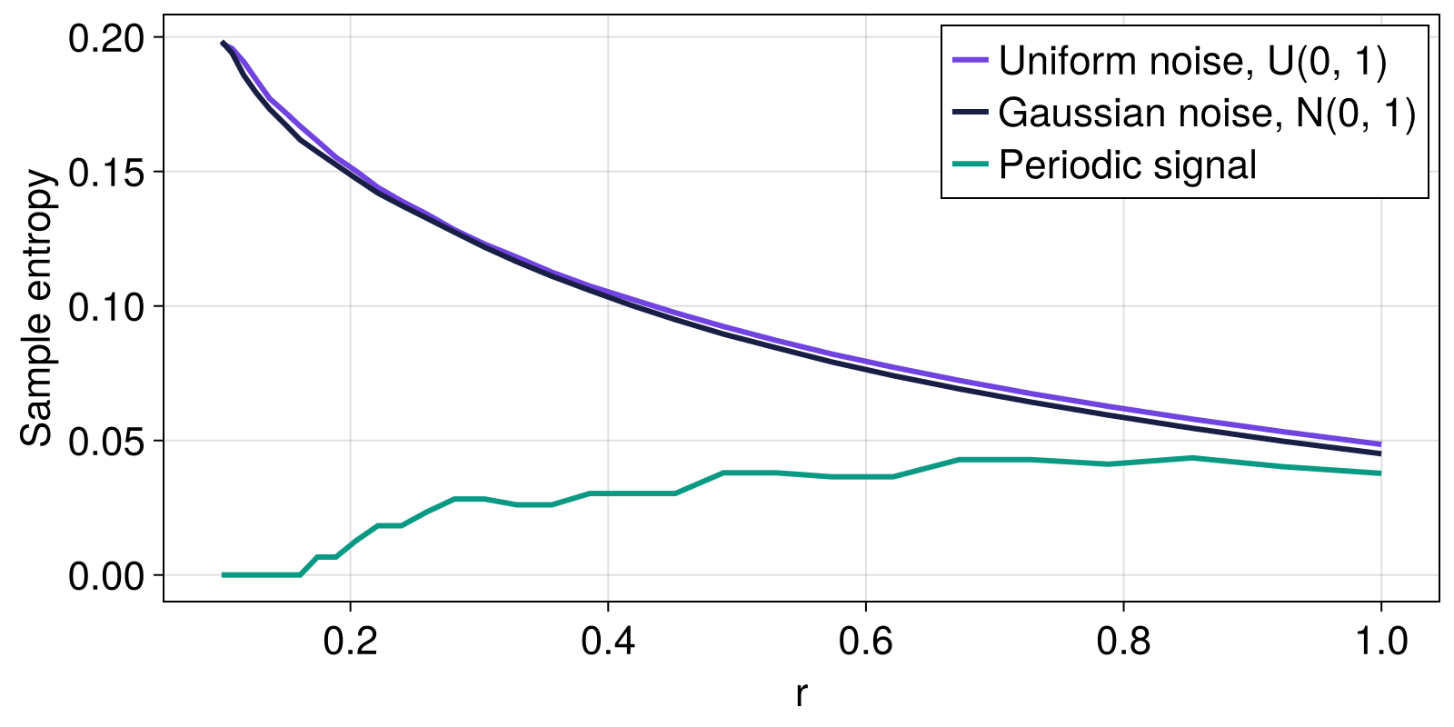

Statistical complexity of iterated maps

In this example, we reproduce parts of Fig. 1 in Rosso et al. (2007): We compute the statistical complexity of the Henon, logistic and Schuster map, as well as that of k-noise.

using ComplexityMeasures
using Distances
using DynamicalSystemsBase
using CairoMakie
using FFTW
using Statistics

N = 2^15

function logistic(x0=0.4; r = 4.0)
    return DeterministicIteratedMap(logistic_rule, SVector(x0), [r])
end
logistic_rule(x, p, n) = @inbounds SVector(p[1]*x[1]*(1 - x[1]))
logistic_jacob(x, p, n) = @inbounds SMatrix{1,1}(p[1]*(1 - 2x[1]))

function henon(u0=zeros(2); a = 1.4, b = 0.3)
    return DeterministicIteratedMap(henon_rule, u0, [a,b])
end
henon_rule(x, p, n) = SVector{2}(1.0 - p[1]*x[1]^2 + x[2], p[2]*x[1])
henon_jacob(x, p, n) = SMatrix{2,2}(-2*p[1]*x[1], p[2], 1.0, 0.0)

function schuster(x0=0.5, z=3.0/2)
    return DeterministicIteratedMap(schuster_rule, SVector(x0), [z])
end
schuster_rule(x, p, n) = @inbounds SVector((x[1]+x[1]^p[1]) % 1)

# generate noise with power spectrum that falls like 1/f^k
function k_noise(k=3)
    function f(N)
        x = rand(Float64, N)
        # generate power spectrum of random numbers and multiply by f^(-k/2)
        x_hat = fft(x) .* abs.(vec(fftfreq(length(x)))) .^ (-k/2)
        # set to zero for frequency zero
        x_hat[1] = 0
        return real.(ifft(x_hat))
    end
    return f
end

fig = Figure()
ax = Axis(fig[1, 1]; xlabel=L"H_S", ylabel=L"C_{JS}")

m, τ = 6, 1
m_kwargs = (
        (color=:transparent,
        strokecolor=:red,
        marker=:utriangle,
        strokewidth=2),
        (color=:transparent,
        strokecolor=:blue,
        marker=:rect,
        strokewidth=2),
        (color=:magenta,
        marker=:circle),
        (color=:blue,
        marker=:rect)
    )

n = 100

c = StatisticalComplexity(
    dist=JSDivergence(),
    est=OrdinalPatterns(; m, τ),
    entr=Renyi()
)
for (j, (ds_gen, sym, ds_name)) in enumerate(zip(
        (logistic, henon, schuster, k_noise),
        (:utriangle, :rect, :dtriangle, :diamond),
        ("Logistic map", "Henon map", "Schuster map", "k-noise (k=3)"),
    ))

    if j < 4
        dim = dimension(ds_gen())
        hs, cs = zeros(n), zeros(n)
        for k in 1:n
            ic = rand(dim) * 0.3
            ds = ds_gen(SVector{dim}(ic))
            x, t = trajectory(ds, N, Ttr=100)
            hs[k], cs[k] = entropy_complexity(c, x[:, 1])
        end
        scatter!(ax, mean(hs), mean(cs); label="$ds_name", markersize=25, m_kwargs[j]...)
    else
        ds = ds_gen()
        hs, cs = zeros(n), zeros(n)
        for k in 1:n
            x = ds(N)
            hs[k], cs[k] = entropy_complexity(c, x[:, 1])
        end
        scatter!(ax, mean(hs), mean(cs); label="$ds_name", markersize=25, m_kwargs[j]...)
    end
end

min_curve, max_curve = entropy_complexity_curves(c)
lines!(ax, min_curve; color=:black)
lines!(ax, max_curve; color=:black)
axislegend(; position=:lt)
fig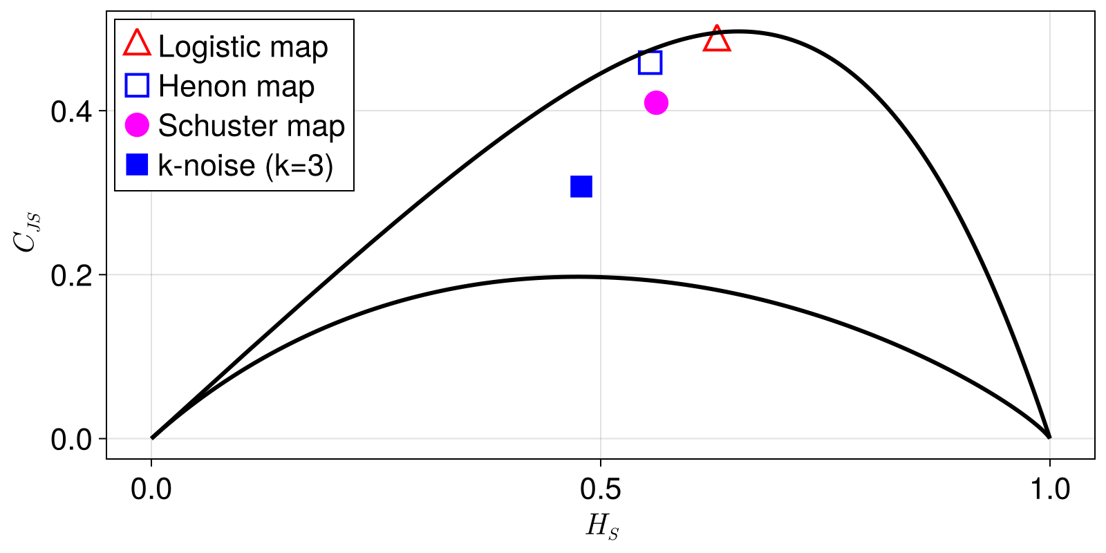

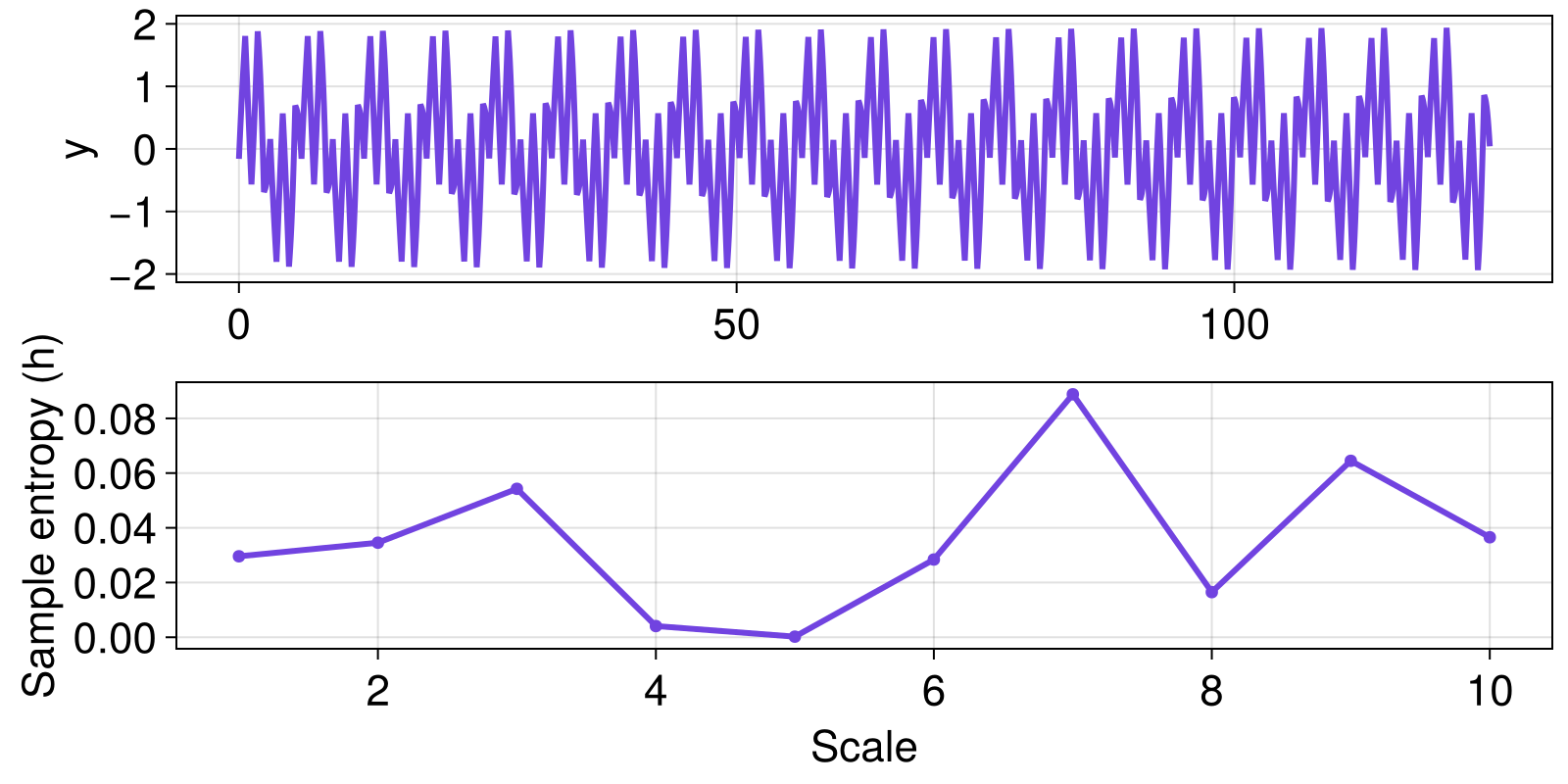
Complexity: multiscale

Let's use multiscale analysis to investigate the SampleEntropy of a signal across coarse-graining scales.

using ComplexityMeasures
using CairoMakie

N, a = 2000, 20
t = LinRange(0, 2*a*π, N)
scales = 1:10

x = repeat([-5:5 |> collect; 4:-1:-4 |> collect], N ÷ 20);
y = sin.(t .+ cos.(t/0.5)) .+ 0.2 .* x
hs = multiscale_normalized(RegularDownsampling(; scales), SampleEntropy(y), y)

fig = Figure()
ax1 = Axis(fig[1,1]; ylabel = "y")
lines!(ax1, t, y; color = Cycled(1));
ax2 = Axis(fig[2, 1]; ylabel = "Sample entropy (h)", xlabel = "Scale")
scatterlines!(ax2, scales |> collect, hs; color = Cycled(1));
fig