Tutorial
The goal of this tutorial is threefold:
- To convey the terminology used by ComplexityMeasures.jl: key terms, what they mean, and how they are used within the codebase.
- To provide a rough overview of the overall features provided by ComplexityMeasures.jl.
- To introduce the main API functions of ComplexityMeasures.jl in a single, self-contained document: how these functions connect to key terms, what are their main inputs and outputs, and how they are used in realistic scientific scripting.
The documentation and exposition of ComplexityMeasures.jl is inspired by chapter 5 of Nonlinear Dynamics, Datseris & Parlitz, Springer 2022 (Datseris and Parlitz, 2022), and expanded to cover more content.
First things first: "complexity measures"
"Complexity measure" is a generic, umbrella term, used extensively in the nonlinear timeseries analysis (NLTS) literature. Roughly speaking, a complexity measure is a quantity extracted from input data that quantifies some dynamical property in the data (often, complexity measures are entropy variants). These complexity measures can highlight some aspects of the dynamics more than others, or distinguish one type of dynamics from another, or classify timeseries into classes with different dynamics, among other things. Typically, more "complex" data have higher complexity measure value. ComplexityMeasures.jl implements hundreds such measures, and hence it is named as such. To enable this, ComplexityMeasures.jl is more than a collection "dynamic statistics": it is also a framework for rigorously defining probability spaces and estimating probabilities from input data.
Within the codebase of ComplexityMeasures.jl we make a separation with the functions information (or its daughter function entropy) and complexity. We use information for complexity measures that are explicit functionals of probability mass or probability density functions, even though these measures might not be labelled as "information measures" in the literature. We use complexity for other complexity measures that are not explicit functionals of probabilities. We stress that the separation between information and complexity is purely pragmatic, to establish a generic and extendable software interface within ComplexityMeasures.jl.
The basics: probabilities and outcome spaces
Information measures and some other complexity measures are computed based on probabilities derived from input data. In order to derive probabilities from data, an outcome space (also called a sample space) needs to be defined: a way to transform data into elements $\omega$ of an outcome space $\omega \in \Omega$, and assign probabilities to each outcome $p(\omega)$, such that $p(\Omega)=1$. $\omega$ are called outcomes or events. In code, outcome spaces are subtypes of OutcomeSpace. For example, one outcome space is the ValueBinning, which is the most commonly known outcome space, and corresponds to discretizing data by putting the data values into bins of a specific size.
using ComplexityMeasures

x = randn(10_000)
ε = 0.1 # bin width
o = ValueBinning(ε)
o isa OutcomeSpacetrueSuch outcome spaces may be given to probabilities_and_outcomes to estimate the probabilities and corresponding outcomes from input data:
probs, outs = probabilities_and_outcomes(o, x);
probs
Probabilities{Float64,1} over 72 outcomes
[-3.7042002010305644] 0.0002
[-3.504200201030564] 0.0001
[-3.3042002010305644] 0.0001
[-3.2042002010305644] 0.0003
[-3.1042002010305643] 0.0003
[-3.004200201030564] 0.0006
[-2.904200201030564] 0.0003
[-2.8042002010305644] 0.0003
[-2.7042002010305644] 0.0012
[-2.6042002010305643] 0.0013
⋮
[2.7957997989694356] 0.0004
[2.895799798969436] 0.0002
[2.995799798969436] 0.0004
[3.0957997989694364] 0.0003
[3.195799798969436] 0.0005
[3.2957997989694356] 0.0001
[3.395799798969436] 0.0002
[3.895799798969436] 0.0001
[4.095799798969436] 0.0001In this example the probabilities are the (normalized) heights of each bin of the histogram. The bins, which are the elements of the outcome space, are shown in the margin, left of the probabilities. They are also returned explicitly as outs above.
This convenience printing syntax with outcomes and probabilities is useful for visual inspection of the probabilities data. However, don't let it worry you. Probabilities are returned as a special Probabilities type that behaves identically to a standard Julia numerical Vector. You can obtain the maximum probability
maximum(probs)0.041or iterate over the probabilities
function total(probs)
    t = 0.0
    for p in probs
        t += p
    end
    return t
end

total(probs)0.9999999999999999Notice that if you use probabilities instead of probabilities_and_outcomes, then outcomes are enumerated generically. This avoids computing outcomes explicitly, and can save some computation time in cases where you don't need the outcomes.
probs2 = probabilities(o, x) Probabilities{Float64,1} over 72 outcomes
Outcome(1) 0.0002
Outcome(2) 0.0001
Outcome(3) 0.0001
Outcome(4) 0.0003
Outcome(5) 0.0003
Outcome(6) 0.0006
Outcome(7) 0.0003
Outcome(8) 0.0003
Outcome(9) 0.0012
Outcome(10) 0.0013
⋮
Outcome(64) 0.0004
Outcome(65) 0.0002
Outcome(66) 0.0004
Outcome(67) 0.0003
Outcome(68) 0.0005
Outcome(69) 0.0001
Outcome(70) 0.0002
Outcome(71) 0.0001
Outcome(72) 0.0001Of course, if the outcomes are obtained for free while estimating the probabilities, they would be included in the return value.
For the ValueBinning example that we use, the outcomes are the left edges of each bin. This allows us to straightforwardly visualize the results.
using CairoMakie
outs = outcomes(probs);
left_edges = only.(outs) # convert `Vector{SVector}` into `Vector{Real}`
barplot(left_edges, probs; axis = (ylabel = "probability",))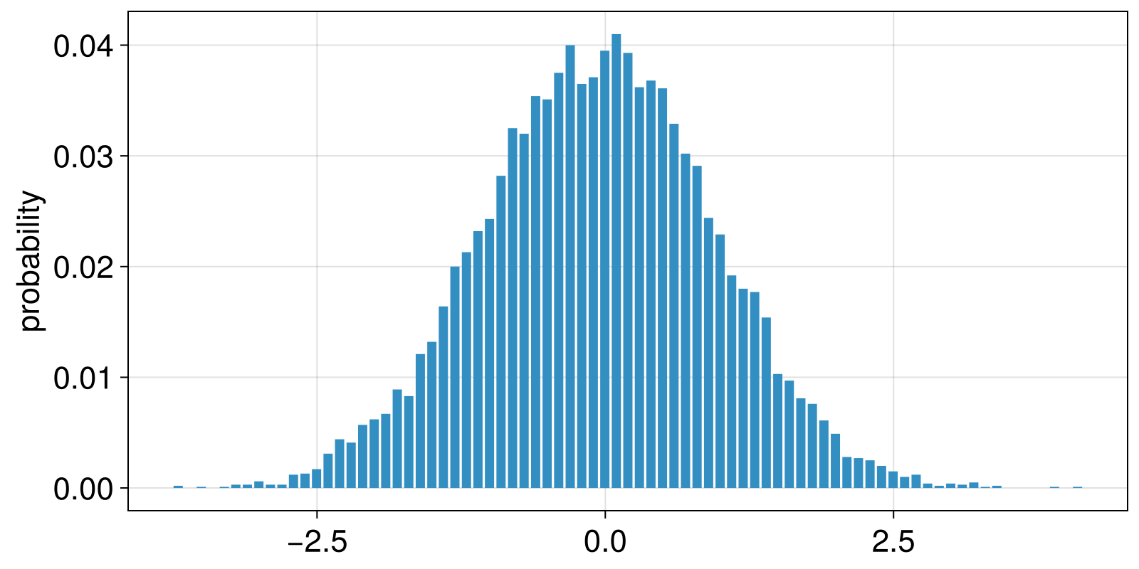
Naturally, there are other outcome spaces one may use, and one can find the list of implemented ones in OutcomeSpace. A prominent example used in the NLTS literature are ordinal patterns. The outcome space for it is OrdinalPatterns, and can be particularly useful with timeseries that come from nonlinear dynamical systems. For example, let's simulate a logistic map timeseries.
using DynamicalSystemsBase

logistic_rule(u, r, t) = SVector(r * u[1] * (1 - u[1]))
ds = DeterministicIteratedMap(logistic_rule, [0.4], 4.0)
Y, t = trajectory(ds, 10_000; Ttr = 100)
y = Y[:, 1]
summary(y)
"10001-element Vector{Float64}"We can then estimate the probabilities corresponding to the ordinal patterns of a certain length (here we use m = 3).
o = OrdinalPatterns{3}()
probsy = probabilities(o, y)
Probabilities{Float64,1} over 5 outcomes
[1, 2, 3] 0.33973397339733974
[1, 3, 2] 0.06440644064406441
[2, 1, 3] 0.13051305130513052
[2, 3, 1] 0.1996199619961996
[3, 1, 2] 0.26572657265726574Comparing these probabilities with those for the purely random timeseries x,
probsx = probabilities(o, x) Probabilities{Float64,1} over 6 outcomes
[1, 2, 3] 0.16583316663332667
[1, 3, 2] 0.16473294658931786
[2, 1, 3] 0.16593318663732748
[2, 3, 1] 0.16873374674934988
[3, 1, 2] 0.16993398679735947
[3, 2, 1] 0.16483296659331867you will notice that the probabilities computing from x has six outcomes, while the probabilities computed from the timeseries y has five outcomes.
The reason that there are less outcomes in the y is because one outcome was never encountered in the y data. This is a common theme in ComplexityMeasures.jl: outcomes that are not in the data are skipped. This can save memory for outcome spaces with large numbers of outcomes. To explicitly obtain all outcomes, by assigning 0 probability to not encountered outcomes, use allprobabilities_and_outcomes. For OrdinalPatterns the outcome space does not depend on input data and is always the same. Hence, the corresponding outcomes matching to allprobabilities_and_outcomes, coincide for x and y, and also coincide with the output of the function outcome_space:
o = OrdinalPatterns()
probsx = allprobabilities(o, x)
probsy = allprobabilities(o, y)
outsx = outsy = outcome_space(o)
# display all quantities as parallel columns
hcat(outsx, probsx, probsy)
6×3 Matrix{Any}:
[1, 2, 3] 0.165833 0.339734
[1, 3, 2] 0.164733 0.0644064
[2, 1, 3] 0.165933 0.130513
[2, 3, 1] 0.168734 0.19962
[3, 1, 2] 0.169934 0.265727
[3, 2, 1] 0.164833 0.0The number of possible outcomes, i.e., the cardinality of the outcome space, can always be found using total_outcomes:
total_outcomes(o)6Beyond the basics: probabilities estimators
So far we have been estimating probabilities by counting the amount of times each possible outcome was encountered in the data, then normalizing. This is called "maximum likelihood estimation" of probabilities. To get the counts themselves, use the counts or counts_and_outcomes function.
countsy = counts(o, y) Counts{Int64,1} over 5 outcomes
Outcome(1) 3397
Outcome(2) 644
Outcome(3) 1305
Outcome(4) 1996
Outcome(5) 2657Counts are printed like Probabilities: they display the outcomes they match to on the left marginal, but otherwise can be used as standard Julia numerical Vectors. To go from outcomes to probabilities, we divide with the total:
probsy = probabilities(o, y)
outsy = outcomes(probsy)
hcat(outsy, countsy, countsy ./ sum(countsy), probsy)
5×4 Matrix{Any}:
[1, 2, 3] 3397 0.339734 0.339734
[1, 3, 2] 644 0.0644064 0.0644064
[2, 1, 3] 1305 0.130513 0.130513
[2, 3, 1] 1996 0.19962 0.19962
[3, 1, 2] 2657 0.265727 0.265727By definition, columns 3 and 4 are identical. However, there are other ways to estimate probabilities that may account for biases in counting outcomes from finite data. Alternative estimators for probabilities are subtypes of ProbabilitiesEstimator. ProbabilitiesEstimators dictate alternative ways to estimate probabilities, given some outcome space and unput data. For example, one could use BayesianRegularization.
probsy_bayes = probabilities(BayesianRegularization(), o, y)

probsy_bayes .- probsy
5-element Vector{Float64}:
-6.98390510782132e-5
6.776967180924243e-5
3.472958251440894e-5
1.8994302469765856e-7
-3.285014627013583e-5While the corrections of BayesianRegularization are small in this case, they are nevertheless measurable.
When calling probabilities only with an outcome space instance and some input data (skipping the ProbabilitiesEstimator), then by default, the RelativeAmount probabilities estimator is used to extract the probabilities.
Entropies
Many compexity measures are a straightforward estimation of Shannon entropy, computed over probabilities estimated from data over some particular outcome space. For example, the well known permutation entropy (Bandt and Pompe, 2002) is exactly the Shannon entropy of the probabilities probsy we computed above based on ordinal patterns. To compute it, we use the entropy function.
perm_ent_x = entropy(OrdinalPatterns(), x)
perm_ent_y = entropy(OrdinalPatterns(), y)
(perm_ent_x, perm_ent_y)
(2.5848619813624496, 2.139506127185978)As expected, the permutation entropy of the x signal is higher, because the signal is "more random". Moreover, since we have estimated the probabilities already, we could have passed these to the entropy function directly instead of recomputing them as above
perm_ent_y_2 = entropy(probsy)2.139506127185978We crucially realize here that many quantities in the NLTS literature that are named as entropies, such as "permutation entropy", are not really new entropies. They are the good old Shannon entropy (Shannon), but calculated with new outcome spaces that smartly quantify some dynamic property in the data. Nevertheless, we acknowledge that names such as "permutation entropy" are commonplace, so in ComplexityMeasures.jl we provide convenience functions like entropy_permutation. More convenience functions can be found in the convenience documentation page.
Beyond Shannon: more entropies
Just like there are different outcome spaces, the same concept applies to entropy. There are many fundamentally different entropies. Shannon entropy is not the only one, just the one used most often. Each entropy is a subtype of InformationMeasure. Another commonly used entropy is the Renyi or generalized entropy. We can use Renyi as an additional first argument to the entropy function to estimate the generalized entropy:
perm_ent_y_q2 = entropy(Renyi(q = 2.0), OrdinalPatterns(), y)
(perm_ent_y_q2, perm_ent_y)
(2.0170680478970375, 2.139506127185978)In fact, when we called entropy(OrdinalPatterns(), y), this dispatched to the default call of entropy(Shannon(), OrdinalPatterns(), y).
Beyond entropies: discrete estimators
The estimation of an entropy truly parallelizes the estimation of probabilities: in the latter, we could decide an outcome space and an estimator to estimate probabilities. The same happens for entropy: we can decide an entropy definition and an estimator of how to estimate the entropy. For example, instead of the default PlugIn estimator that we used above implicitly, we could use the Jackknife estimator.
ospace = OrdinalPatterns()
entdef = Renyi(q = 2.0)
entest = Jackknife(entdef)
perm_ent_y_q2_jack = entropy(entest, ospace, y)

(perm_ent_y_q2, perm_ent_y_q2_jack)
(2.0170680478970375, 1.2173088128474774)Entropy estimators always reference an entropy definition, even if they only apply to one type of entropy (typically the Shannon one). From here, it is up to the researcher to read the documentation of the plethora of estimators implemented and decide what is most suitable for their data at hand. They all can be found in DiscreteInfoEstimator.
Beyond entropies: other information measures
Recall that at the very beginning of this notebook we mentioned a code separation of information and complexity. We did this because there are other measures, besides entropy, that are explicit functionals of some probability mass function. One example is the Shannon extropy ShannonExtropy, the complementary dual of entropy, which could be computed as follows.
extdef = ShannonExtropy()
perm_ext_y = information(extdef, ospace, y)1.2450281736700084Just like the Shannon entropy, the extropy could also be estimated with a different estimator such as Jackknife.
perm_ext_y_jack = information(Jackknife(extdef), ospace, y)1.126229249906828In truth, when we called entropy(e, o, y) it actually calls information(e, o, y), as all "information measures" are part of the same function interface. And entropy is an information measure.
Beyond discrete: differential or continuous
Discrete information measures are functions of probability mass functions. It is also possible to compute information measures of probability density functions. In ComplexityMeasures.jl, this is done by calling entropy (or the more general information) with a differential information estimator, a subtype of DifferentialInfoEstimator. These estimators are given directly to information without assigning an outcome space, because the probability density is approximated implicitly, not explicitly. For example, the Correa estimator approximates the differential Shannon entropy by utilizing order statistics of the timeseries data:
diffest = Correa()
diffent = entropy(diffest, x)1.7961913255195951Beyond information: other complexity measures
As discussed at the very beginning of this tutorial, there are some complexity measures that are not explicit functionals of probabilities, and hence cannot be straightforwardly related to an outcome space, in the sense of providing an instance of OutcomeSpace to the estimation function. These are estimated with the complexity function, by providing it a subtype of ComplexityEstimator. An example here is the well-known sample entropy (which isn't actually an entropy in the formal mathematical sense). It can be computed as follows.
complest = SampleEntropy(r = 0.1)
sampent = complexity(complest, y)
0.612355215298896