Defining a forced dynamical system
This section explains how to specify your dynamical system and forcing of interest.
To specify a system, CriticalTransitions provides three core system types:
- CoupledODEs - used to define a deterministic system of ordinary differential equations of the form $\frac{\text{d}\mathbf{u}}{\text{d}t} = \mathbf{f}(\mathbf{u}, p, t)$.
- CoupledSDEs - used to define a system of stochastic differential equations of the form $\text{d}\mathbf{u} = \mathbf{f}(\mathbf{u}, p, t) \text{d}t + \mathbf{g}(\mathbf{u}, p, t) \text{d}\mathcal{N}_t$.
- RateSystem - used to define a non-autonomous system with parametric forcing of the form $\frac{\text{d}\mathbf{u}}{\text{d}t} = \mathbf{f}(\mathbf{u}(t), p(t))$.
The CoupledODEs and CoupledSDEs system types are inherited from DynamicalSystemsBase.jl. The RateSystem type is added in CriticalTransitions.jl to enable easy construction of non-autonomous dynamical systems in which a parameter changes over time.
Deterministic: CoupledODEs
DynamicalSystemsBase.CoupledODEs — Type
CoupledODEs <: ContinuousTimeDynamicalSystem
CoupledODEs(f, u0 [, p]; diffeq, t0 = 0.0)
A deterministic continuous time dynamical system defined by a set of coupled ordinary differential equations as follows:
\[\frac{d\vec{u}}{dt} = \vec{f}(\vec{u}, p, t)\]
An alias for CoupledODE is ContinuousDynamicalSystem.
Optionally provide the parameter container p and initial time as keyword t0.
For construction instructions regarding f, u0 see the DynamicalSystems.jl tutorial.
DifferentialEquations.jl interfacing
The ODEs are evolved via the solvers of DifferentialEquations.jl. When initializing a CoupledODEs, you can specify the solver that will integrate f in time, along with any other integration options, using the diffeq keyword. For example you could use diffeq = (abstol = 1e-9, reltol = 1e-9). If you want to specify a solver, do so by using the keyword alg, e.g.: diffeq = (alg = Tsit5(), reltol = 1e-6). This requires you to have been first using OrdinaryDiffEq (or smaller library package such as OrdinaryDiffEqVerner) to access the solvers. The default diffeq is:
(alg = OrdinaryDiffEqTsit5.Tsit5{typeof(OrdinaryDiffEqCore.triviallimiter!), typeof(OrdinaryDiffEqCore.triviallimiter!), FastBroadcast.Serial}(OrdinaryDiffEqCore.triviallimiter!, OrdinaryDiffEqCore.triviallimiter!, FastBroadcast.Serial()), abstol = 1.0e-6, reltol = 1.0e-6)
diffeq keywords can also include callback for event handling .
The convenience constructors CoupledODEs(prob::ODEProblem [, diffeq]) and CoupledODEs(ds::CoupledODEs [, diffeq]) are also available. Use ODEProblem(ds::CoupledODEs, tspan = (t0, Inf)) to obtain the problem.
To integrate with ModelingToolkit.jl, the dynamical system must be created via the ODEProblem (which itself is created via ModelingToolkit.jl), see the Tutorial for an example.
Dev note: CoupledODEs is a light wrapper of ODEIntegrator from DifferentialEquations.jl.
Stochastic: CoupledSDEs
DynamicalSystemsBase.CoupledSDEs — Type
CoupledSDEs <: ContinuousTimeDynamicalSystem
CoupledSDEs(f, u0 [, p]; kwargs...)
A stochastic continuous time dynamical system defined by a set of coupled stochastic differential equations (SDEs) as follows:
\[\text{d}\mathbf{u} = \mathbf{f}(\mathbf{u}, p, t) \text{d}t + \mathbf{g}(\mathbf{u}, p, t) \text{d}\mathcal{N}_t\]
where $\mathbf{u}(t)$ is the state vector at time $t$, $\mathbf{f}$ describes the deterministic dynamics, and the noise term $\mathbf{g}(\mathbf{u}, p, t) \text{d}\mathcal{N}_t$ describes the stochastic forcing in terms of a noise function (or diffusion function) $\mathbf{g}$ and a noise process $\mathcal{N}_t$. The parameters of the functions $\mathcal{f}$ and $\mathcal{g}$ are contained in the vector $p$.
There are multiple ways to construct a CoupledSDEs depending on the type of stochastic forcing.
The only required positional arguments are the deterministic dynamic rule f(u, p, t), the initial state u0, and optinally the parameter container p (by default p = nothing). For construction instructions regarding f, u0 see the DynamicalSystems.jl tutorial .
By default, the noise term is standard Brownian motion, i.e. additive Gaussian white noise with identity covariance matrix. To construct different noise structures, see below.
Noise term
The noise term can be specified via several keyword arguments. Based on these keyword arguments, the noise function g is constructed behind the scenes unless explicitly given.
- The noise strength (i.e. the magnitude of the stochastic forcing) can be scaled with
noise_strength(defaults to1.0). This factor is multiplied with the whole noise term. - For non-diagonal and correlated noise, a covariance matrix can be provided via
covariance(defaults to identity matrix of sizelength(u0).) - For more complicated noise structures, including state- and time-dependent noise, the noise function
gcan be provided explicitly as a keyword argument (defaults tonothing). For construction instructions, continue reading.
The function g interfaces to the diffusion function specified in an SDEProblem of DynamicalSystems.jl. g must follow the same syntax as f, i.e., g(u, p, t) for out-of-place (oop) and g!(du, u, p, t) for in-place (iip).
Unless g is of vector form and describes diagonal noise, a prototype type instance for the output of g must be specified via the keyword argument noise_prototype. It can be of any type A that has the method LinearAlgebra.mul!(Y, A, B) -> Y defined. Commonly, this is a matrix or sparse matrix. If this is not given, it defaults to nothing, which means the g should be interpreted as being diagonal.
The noise process can be specified via noise_process. It defaults to a standard Wiener process (Gaussian white noise). For details on defining noise processes, see the docs of DiffEqNoiseProcess.jl . A complete list of the pre-defined processes can be found here. Note that DiffEqNoiseProcess.jl also has an interface for defining custom noise processes.
By combining g and noise_process, you can define different types of stochastic systems. Examples of different types of stochastic systems are listed on the StochasticDiffEq.jl tutorial page. A quick overview of common types of stochastic systems can also be found in the online docs for CoupledSDEs.
Keyword arguments
g: noise function (defaultnothing)noise_strength: scaling factor for noise strength (default1.0)covariance: noise covariance matrix (defaultnothing)noise_prototype: prototype instance for the output ofg(defaultnothing)noise_process: stochastic process as provided by DiffEqNoiseProcess.jl (defaultnothing, i.e. standard Wiener process)t0: initial time (default0.0)diffeq: DiffEq solver settings (see below)seed: random number seed (defaultrand(UInt64), so eachCoupledSDEsproduces a different noise realization unless a seed is given explicitly)
DifferentialEquations.jl interfacing
The CoupledSDEs is evolved using the solvers of DifferentialEquations.jl. To specify a solver via the diffeq keyword argument, use the flag alg, which can be accessed after loading StochasticDiffEq.jl (using StochasticDiffEq). The default diffeq is:
(alg = SOSRA(), abstol = 1.0e-2, reltol = 1.0e-2)diffeq keywords can also include a callback for event handling .
Dev note: CoupledSDEs is a light wrapper of SDEIntegrator from StochasticDiffEq.jl. The integrator is available as the field integ, and the SDEProblem is integ.sol.prob. The convenience syntax SDEProblem(ds::CoupledSDEs, tspan = (t0, Inf)) is available to extract the problem.
Converting between CoupledSDEs and CoupledODEs
You can convert a CoupledSDEs system to CoupledODEs to analyze its deterministic part using the function CoupledODEs(ds::CoupledSDEs; diffeq, t0). Similarly, use CoupledSDEs(ds::CoupledODEs [, p]; kwargs...) to convert a CoupledODEs into a CoupledSDEs.
Check out some examples of how to construct different types of stochastic dynamics here.
Note that nonlinear mixings of the Noise Process $\mathcal{W}$ fall into the class of random ordinary differential equations (RODEs) which have a separate set of solvers. See this example of DifferentialEquations.jl.
CoupledSDEs API
CriticalTransitions.solver — Function
solver(ds::ContinuousTimeDynamicalSystem) -> Any
Returns the SDE solver specified in the diffeq settings of the CoupledSDEs.
CriticalTransitions.drift — Function
drift(
    sys::Union{CoupledODEs{IIP}, CoupledSDEs{IIP}},
    x;
    t
) -> Any
Returns the deterministic drift $f(x)$ of the CoupledSDEs sys at state x. For time-dependent systems, the time can be specified as a keyword argument t (by default t=0).
CriticalTransitions.div_drift — Function
div_drift(sys::ContinuousTimeDynamicalSystem, x) -> Any
div_drift(sys::ContinuousTimeDynamicalSystem, x, t) -> Any
Computes the divergence of the drift field $f(x)$ at state x. For time- dependent systems, the time can be specified as a keyword argument t (by default t=0).
DynamicalSystemsBase.covariance_matrix — Function
covariance_matrix(ds::CoupledSDEs)Returns the covariance matrix of the stochastic term of the CoupledSDEs ds, provided that the diffusion function g can be expressed as a constant invertible matrix. If this is not the case, returns nothing.
See also diffusion_matrix.
DynamicalSystemsBase.diffusion_matrix — Function
diffusion_matrix(ds::CoupledSDEs)Returns the diffusion matrix of the stochastic term of the CoupledSDEs ds, provided that the diffusion function g can be expressed as a constant invertible matrix. If this is not the case, returns nothing.
Note: The diffusion matrix $Σ$ is the square root of the noise covariance matrix $Q$ (see covariance_matrix), defined via the Cholesky decomposition $Q = Σ Σ^\top$.
CriticalTransitions.noise_process — Function
noise_process(sys::CoupledSDEs) -> Any
Fetches the stochastic process $\mathcal{N}$ specified in the intergrator of sys. Returns the type DiffEqNoiseProcess.NoiseProcess.
CriticalTransitions.noise_strength — Function
noise_strength(sys::CoupledSDEs) -> Any
Effective noise strength $\sigma_{\mathrm{eff}} = \sqrt{\mathrm{tr}(\mathbf{\Sigma})/D}$ of sys, where $\mathbf{\Sigma} =$ covariance_matrix(sys) and $D =$ dimension(sys). Together with normalize_covariance! it satisfies $\sigma_{\mathrm{eff}}^2 \cdot \mathbf{Q}_{\mathrm{can}} = \mathbf{\Sigma}$.
For an SDE built as $\mathrm{d}\mathbf{x} = \mathbf{b}\,\mathrm{d}t + \sigma\sqrt{\mathbf{Q}}\,\mathrm{d}\mathbf{W}$:
- Isotropic
covariance = c·I: $\sigma_{\mathrm{eff}} = \sigma\sqrt{c}$. The defaultcovariance = I($c=1$) recovers the construction-timenoise_strengthkeyword exactly. - Anisotropic
Q: $\sigma_{\mathrm{eff}} = \sigma\sqrt{\mathrm{tr}(\mathbf{Q})/D}$, the per-direction average noise amplitude. Equals $\sigma$ whenever $\mathrm{tr}(\mathbf{Q}) = D$. - Custom
g(not of the form $\sigma\sqrt{\mathbf{Q}}$): still well-defined as the trace-based effective σ of the resulting $\mathbf{\Sigma}$.
See Large deviation theory for the role of $\sigma_{\mathrm{eff}}$ in the action functionals.
Noise strength and the trace convention
A CoupledSDEs exposes its noise via the diffusion function $g$ and, for additive invertible noise, the noise rate covariance
\[\mathbf{\Sigma} \;=\; \texttt{covariance\_matrix(sys)} \;=\; g\,g^\top.\]
For an SDE built as $\mathrm{d}\mathbf{x} = \mathbf{b}\,\mathrm{d}t + \sigma\,\mathbf{\Sigma}_0\,\mathrm{d}\mathbf{W}_t$ with $\mathbf{\Sigma}_0\mathbf{\Sigma}_0^\top = \mathbf{Q}$, this gives $\mathbf{\Sigma} = \sigma^2\,\mathbf{Q}$.
The noise strength and the covariance are not separately determined by the SDE: only their product $\sigma^2\mathbf{Q}$ enters, and $(\sigma, \mathbf{Q}) \leftrightarrow (c\sigma, \mathbf{Q}/c^2)$ describes the same physical system. The package picks a unique $(\sigma, \mathbf{Q})$ pair from $\mathbf{\Sigma}$ by adopting the trace convention $\mathrm{tr}(\mathbf{Q}) = D$:
\[\sigma_{\mathrm{eff}}^2 \;=\; \frac{\mathrm{tr}(\mathbf{\Sigma})}{D}, \qquad \mathbf{Q}_{\mathrm{can}} \;=\; \frac{D}{\mathrm{tr}(\mathbf{\Sigma})}\,\mathbf{\Sigma}.\]
The accessor noise_strength(sys) returns $\sigma_{\mathrm{eff}}$. The trace is invariant under orthogonal changes of basis and reduces to the per-direction average noise variance, making this the natural choice among rotation-invariant normalizations.
This convention is what the large deviation action functionals use: they evaluate the Freidlin-Wentzell integrand in the $\mathbf{Q}_{\mathrm{can}}^{-1}$ metric,
\[\texttt{fw\_action(sys, path, time)} \;=\; \Phi_{FW}^{\mathbf{Q}_{\mathrm{can}}}[\phi] \;=\; \tfrac{1}{2}\!\int (\dot\phi - \mathbf{b})^\top \mathbf{Q}_{\mathrm{can}}^{-1}(\dot\phi - \mathbf{b})\,\mathrm{d}t,\]
so the returned action is independent of the noise_strength keyword chosen at construction and invariant under orthogonal changes of basis.
If you built your system as $\mathrm{d}\mathbf{x} = \mathbf{b}\,\mathrm{d}t + \sigma_{\mathrm{user}}\,\mathbf{\Sigma}_0\,\mathrm{d}\mathbf{W}_t$ with $\mathbf{Q}_{\mathrm{user}} = \mathbf{\Sigma}_0\mathbf{\Sigma}_0^\top$ and want the action in your metric $\mathbf{Q}_{\mathrm{user}}^{-1}$, multiply the returned action by $\mathrm{tr}(\mathbf{Q}_{\mathrm{user}})/D$:
\[\Phi_{FW}^{\mathbf{Q}_{\mathrm{user}}}[\phi] \;=\; \frac{\mathrm{tr}(\mathbf{Q}_{\mathrm{user}})}{D}\cdot \texttt{fw\_action(sys, path, time)}.\]
The factor is $1$ whenever $\mathbf{Q}_{\mathrm{user}}$ is isotropic ($c\,\mathbf{I}$ for any $c>0$) or already trace-normalized ($\mathrm{tr}(\mathbf{Q}_{\mathrm{user}}) = D$), in which case fw_action returns $\Phi_{FW}^{\mathbf{Q}_{\mathrm{user}}}$ directly. All examples and tests in the package fall in this case.
Non-autonomous: RateSystem
CriticalTransitions.RateSystem — Type
RateSystem <: ContinuousTimeDynamicalSystem
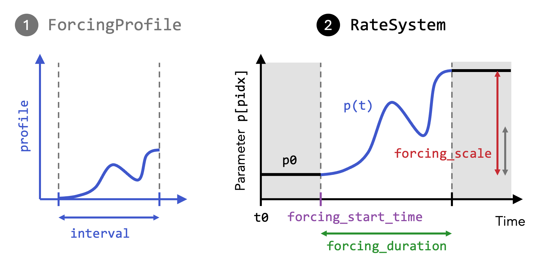
RateSystem(ds::ContinuousTimeDynamicalSystem, forcing_profile::AbstractDict; kw...)Construct a non-autonomous dynamical system by applying time-dependent parametric forcing protocols to an underlying autonomous continuous-time dynamical system ds. The unforced system parameters are copied and are always considered the starting parameter values irrespectively of what happens with ds afterwards.
forcing_profile is a Dict mapping parameter indices (anything valid for set_parameter!) to ForcingProfile instances. Each entry defines the functional form of how the corresponding parameter evolves over time. The profile is then combined with how long, and how large, each parameter forcing is, using the keywords below.
Keyword arguments
forcing_start_time = initial_time(ds): start time(s) for the parameter ramping. You may supply anAbstractDictmapping keys to start times, or a scalar value which will be applied to all forcing profiles.forcing_duration = one(initial_time(ds)): duration of the parameter ramping (in system time units). Can be anAbstractDictmapping keys to durations or a scalar applied to all forcing profiles.forcing_scale = 1.0: amplitude multiplicative factor of the forcing profile. Can be anAbstractDictmapping keys to scales or a scalar applied to all forcing profiles.reverse = false: whether to reverse the forcing after the first forcing interval. Can be anAbstractDictmapping keys to booleans or a scalar boolean applied to all forcing profiles. If true, forcing is reversed over a second interval with the same duration.t0 = initial_time(ds): initial time of theRateSystem.
Description
The profile interval defines the domain of the forcing function; when applied to the system the profile is rescaled in system time units using the configured start and duration values - this allow changing the rate of the parameter ramping. Before a forcingprofile's start time the parameter equals its initial autonomous value; during the forcing interval it follows the rescaled profile (multiplied by the corresponding `forcingscalefactor). Ifreverse = true, the same profile is traversed backwards over a second interval of equal duration, after which the parameter returns to its initial autonomous value. Ifreverse = false`, after the interval the parameter is frozen at its final value.
To modify a rate system after it has been created, use set_forcing_duration!, set_forcing_scale!, set_forcing_start!, set_forcing_reverse!, and to obtain time dependent parameters use parameters, parameter.
Single parameter
You can use the convenience syntax
RateSystem(ds::ContinuousTimeDynamicalSystem, fp::ForcingProfile, pidx; kw...)if you are only varying a single parameter with index pidx.
CriticalTransitions.ForcingProfile — Type
ForcingProfile(profile::Function, interval)Time-dependent forcing profile $p(t)$ describing the evolution of a parameter over a domain interval = (start, end). Used to define a parametric forcing when constructing a non-autonomous RateSystem.
Arguments
profile: function $p(t)$ from $ℝ → ℝ$ describing the parameter changeinterval: domain interval over which theprofileis considered
Note: The units of $t$ are arbitrary; the forcing profile is rescaled to system time units.
Convenience functions
ForcingProfile(:linear): Create a linear ramp from 0 to 1.ForcingProfile(:tanh): Create a hyperbolic tangent ramping from 0 to 1 with interval (-3, 3).
CriticalTransitions.unforced_system — Function
unforced_system(rs::RateSystem, t) -> Any
Returns an autonomous dynamical system corresponding to the frozen system of the non-autonomous RateSystem rs at time t.
RateSystem API
CriticalTransitions.parameters — Function
parameters(rs::RateSystem, t)Return the parameter container of a RateSystem at time t (in system time units). This function returns a non-aliased copy but also modifies the parameter state of rs to be on time t.
CriticalTransitions.parameter — Function
parameter(rs::RateSystem, t, pkey)Returns the parameter with key pkey of a RateSystem at time t (in system time units).
CriticalTransitions.set_forcing_start! — Function
set_forcing_start!(
    rs::RateSystem,
    start_time;
    pkey
) -> RateSystem
Sets the start time (forcing_start_time) of the forcing protocol applied to the RateSystem rs. If the optional keyword pkey is provided, only the start time for that parameter is changed; otherwise all parameters are updated.
CriticalTransitions.set_forcing_duration! — Function
set_forcing_duration!(
    rs::RateSystem,
    duration;
    pkey
) -> RateSystem
Sets the duration (forcing_duration) of the forcing protocol applied to the RateSystem rs. If the optional keyword pkey is provided, only the duration for that parameter is changed; otherwise all parameters are updated.
CriticalTransitions.set_forcing_scale! — Function
set_forcing_scale!(rs::RateSystem, scale; pkey=nothing)Sets the amplitude (forcing_scale) of the forcing of the RateSystem to scale. If the keyword pkey is provided, only the corresponding parameter's forcing scale is changed; otherwise the forcing scale of all parameters is updated to scale.
Converting between systems
The deterministic part of a CoupledSDEs can be extracted as a CoupledODEs, making it compatible with functionality of DynamicalSystems.jl. In turn, a CoupledODEs can easily be extended into a CoupledSDEs.
DynamicalSystemsBase.CoupledODEs — Method
CoupledODEs(ds::CoupledSDEs; kwargs...)Converts a CoupledSDEs into a CoupledODEs by extracting the deterministic part of ds.
DynamicalSystemsBase.CoupledSDEs — Method
CoupledSDEs(ds::CoupledODEs, p = current_parameters(ds); kwargs...)Converts a CoupledODEs into a CoupledSDEs. While p is optional, it is likely to change as the diffusion (noise) function g is added.
For example, the Lyapunov spectrum of a CoupledSDEs in the absence of noise, here exemplified by the FitzHugh-Nagumo model, can be computed by typing:
using CriticalTransitions
using ChaosTools: lyapunovspectrum

function fitzhugh_nagumo(u, p, t)
    x, y = u
    ϵ, β = p
    dx = (-x^3 + x - y)/ϵ
    dy = -β*y + x
    return SVector{2}([dx, dy])
end

p = [1.,3.]

# Define the CoupledSDEs
sys = CoupledSDEs(fitzhugh_nagumo, ones(2), p; noise_strength=0.1)

# Compute Lyapunov spectrum of deterministic flow
ls = lyapunovspectrum(CoupledODEs(sys), 10000)
2-element Vector{Float64}:
0.0037846226653203657
-0.028280268988271094