Overarching tutorial for DynamicalSystems.jl
This page serves as a short but to-the-point introduction to the DynamicalSystems.jl library. It outlines the core components, and how they establish an interface that is used by the rest of the library. It also provides a couple of usage examples to connect the various subpackages of the library together. This is not an in-depth tutorial, and the individual subpackages of the library have their own in-depth tutorials and documentation (see the top bar of the online documentation).
Going through this tutorial should take you about 20-30 minutes.
This tutorial is also available online as a Jupyter notebook.
Installation
To install DynamicalSystems.jl, simply do:
using Pkg; Pkg.add("DynamicalSystems")This installs several packages for the Julia language. Some of these are the sub-modules/packages that comprise DynamicalSystems.jl, see contents for more. All of the functionality is brought into scope when doing:
using DynamicalSystemsin your Julia session.
Package versions used
import Pkg

Pkg.status(["DynamicalSystems", "CairoMakie", "OrdinaryDiffEq", "BenchmarkTools"]; mode = Pkg.PKGMODE_MANIFEST)
Status `~/work/DynamicalSystems.jl/DynamicalSystems.jl/docs/Manifest.toml`
[6e4b80f9] BenchmarkTools v1.6.3
[13f3f980] CairoMakie v0.15.7
[61744808] DynamicalSystems v3.6.5 [loaded: v3.6.6]
[1dea7af3] OrdinaryDiffEq v6.103.0Core components
The individual packages that compose DynamicalSystems interact flawlessly with each other because of the following two components:
- The
StateSpaceSet, which represents numerical data. They can be observed or measured from experiments, sampled trajectories of dynamical systems, or just unordered sets in a state space. AStateSpaceSetis a container of equally-sized points, representing multivariate timeseries or multivariate datasets. Timeseries, which are univariate sets, are represented by theAbstractVector{<:Real}Julia base type. - The
DynamicalSystem, which is the abstract representation of a dynamical system with a known dynamic evolution rule.DynamicalSystemdefines an extendable interface, but typically one uses existing implementations such asDeterministicIteratedMaporCoupledODEs.
Making dynamical systems
In the majority of cases, to make a dynamical system one needs three things:
- The dynamic rule
f: A Julia function that provides the instructions of how to evolve the dynamical system in time. - The state
u: An array-like container that contains the variables of the dynamical system and also defines the starting state of the system. - The parameters
p: An arbitrary container that parameterizesf.
For most concrete implementations of DynamicalSystem there are two ways of defining f, u. The distinction is done on whether f is defined as an in-place (iip) function or out-of-place (oop) function.
- oop :
fmust be in the formf(u, p, t) -> outwhich means that given a stateu::SVector{<:Real}and some parameter containerpit returns the output offas anSVector{<:Real}(static vector). - iip :
fmust be in the formf!(out, u, p, t)which means that given a stateu::AbstractArray{<:Real}and some parameter containerp, it writes in-place the output offinout::AbstractArray{<:Real}. The function must returnnothingas a final statement.
t stands for current time in both cases. iip is suggested for systems with high dimension and oop for small. The break-even point is between 10 to 100 dimensions but should be benchmarked on a case-by-case basis as it depends on the complexity of f.
Whether the dynamical system is autonomous (f doesn't depend on time) or not, it is still necessary to include t as an argument to f. Some algorithms utilize this information, some do not, but we prefer to keep a consistent interface either way.
It is not immediatelly obvious, but all library functions that obtain as an input a DynamicalSystem instance will modify it, in-place. For example the current_state of the system before and after giving it to a function such as basins_of_attraction will not be the same! This also affects parallelization, see below.
Example: Henon map
Let's make the Henon map, defined as
\[\begin{aligned} x_{n+1} &= 1 - ax^2_n+y_n \\ y_{n+1} & = bx_n \end{aligned}\]
with parameters $a = 1.4, b = 0.3$.
First, we define the dynamic rule as a standard Julia function. Since the dynamical system is only two-dimensional, we should use the out-of-place form that returns an SVector with the next state:
using DynamicalSystems

function henon_rule(u, p, n) # here `n` is "time", but we don't use it.
    x, y = u # system state
    a, b = p # system parameters
    xn = 1.0 - a*x^2 + y
    yn = b*x
    return SVector(xn, yn)
end
henon_rule (generic function with 1 method)Then, we define initial state and parameters
u0 = [0.2, 0.3]
p0 = [1.4, 0.3]
2-element Vector{Float64}:
1.4
0.3Lastly, we give these three to the DeterministicIteratedMap:
henon = DeterministicIteratedMap(henon_rule, u0, p0)2-dimensional DeterministicIteratedMap
deterministic: true
discrete time: true
in-place: false
dynamic rule: henon_rule
parameters: [1.4, 0.3]
time: 0
state: [0.2, 0.3]
henon is a DynamicalSystem, one of the two core structures of the library. They can evolved interactively, and queried, using the interface defined by DynamicalSystem. The simplest thing you can do with a DynamicalSystem is to get its trajectory:
total_time = 10_000
X, t = trajectory(henon, total_time)
X
2-dimensional StateSpaceSet{Float64} with 10001 points
0.2 0.3
1.244 0.06
-1.10655 0.3732
-0.341035 -0.331965
0.505208 -0.102311
0.540361 0.151562
0.742777 0.162108
0.389703 0.222833
1.01022 0.116911
-0.311842 0.303065
⋮
-0.582534 0.328346
0.853262 -0.17476
-0.194038 0.255978
1.20327 -0.0582113
-1.08521 0.36098
-0.287758 -0.325562
0.558512 -0.0863275
0.476963 0.167554
0.849062 0.143089X is a StateSpaceSet, the second of the core structures of the library. We'll see below how, and where, to use a StateSpaceset, but for now let's just do a scatter plot
using CairoMakie
scatter(X)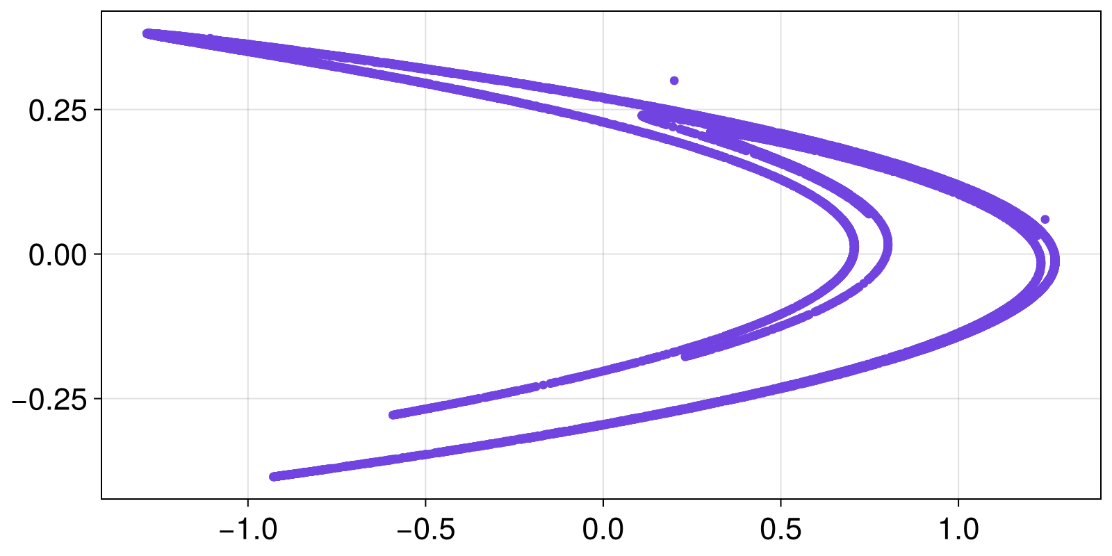
Example: Lorenz96
Let's also make another dynamical system, the Lorenz96 model:
\[\frac{dx_i}{dt} = (x_{i+1}-x_{i-2})x_{i-1} - x_i + F\]
for $i \in \{1, \ldots, N\}$ and $N+j=j$.
Here, instead of a discrete time map we have $N$ coupled ordinary differential equations. However, creating the dynamical system works out just like above, but using CoupledODEs instead of DeterministicIteratedMap.
First, we make the dynamic rule function. Since this dynamical system can be arbitrarily high-dimensional, we prefer to use the in-place form for f, overwriting in place the rate of change in a pre-allocated container. It is customary to append the name of functions that modify their arguments in-place with a bang (!).
function lorenz96_rule!(du, u, p, t)
    F = p[1]; N = length(u)
    # 3 edge cases
    du[1] = (u[2] - u[N - 1]) * u[N] - u[1] + F
    du[2] = (u[3] - u[N]) * u[1] - u[2] + F
    du[N] = (u[1] - u[N - 2]) * u[N - 1] - u[N] + F
    # then the general case
    for n in 3:(N - 1)
        du[n] = (u[n + 1] - u[n - 2]) * u[n - 1] - u[n] + F
    end
    return nothing # always `return nothing` for in-place form!
end
lorenz96_rule! (generic function with 1 method)then, like before, we define an initial state and parameters, and initialize the system
N = 6
u0 = range(0.1, 1; length = N)
p0 = [8.0]
lorenz96 = CoupledODEs(lorenz96_rule!, u0, p0)
6-dimensional CoupledODEs
deterministic: true
discrete time: false
in-place: true
dynamic rule: lorenz96_rule!
ODE solver: Tsit5
ODE kwargs: (abstol = 1.0e-6, reltol = 1.0e-6)
parameters: [8.0]
time: 0.0
state: [0.1, 0.28, 0.46, 0.64, 0.82, 1.0]
and, again like before, we may obtain a trajectory the same way
total_time = 12.5
sampling_time = 0.02
Y, t = trajectory(lorenz96, total_time; Ttr = 2.2, Δt = sampling_time)
Y
6-dimensional StateSpaceSet{Float64} with 626 points
3.15368 -4.40493 0.0311581 0.486735 1.89895 4.15167
2.71382 -4.39303 0.395019 0.66327 2.0652 4.32045
2.25088 -4.33682 0.693967 0.879701 2.2412 4.46619
1.7707 -4.24045 0.924523 1.12771 2.42882 4.58259
1.27983 -4.1073 1.08656 1.39809 2.62943 4.66318
0.785433 -3.94005 1.18319 1.6815 2.84384 4.70147
0.295361 -3.74095 1.2205 1.96908 3.07224 4.69114
-0.181932 -3.51222 1.20719 2.25296 3.3139 4.62628
-0.637491 -3.25665 1.154 2.5267 3.56698 4.50178
-1.06206 -2.9781 1.07303 2.7856 3.82827 4.31366
⋮ ⋮
3.17245 2.3759 3.01796 7.27415 7.26007 -0.116002
3.29671 2.71146 3.32758 7.5693 6.75971 -0.537853
3.44096 3.09855 3.66908 7.82351 6.13876 -0.922775
3.58387 3.53999 4.04452 8.01418 5.39898 -1.25074
3.70359 4.03513 4.45448 8.1137 4.55005 -1.5042
3.78135 4.57879 4.89677 8.09013 3.61125 -1.66943
3.80523 5.16112 5.36441 7.90891 2.61262 -1.73822
3.77305 5.7684 5.84318 7.53627 1.59529 -1.71018
3.6934 6.38507 6.30923 6.94454 0.61023 -1.59518We can't scatterplot something 6-dimensional but we can visualize all timeseries
fig = Figure()
ax = Axis(fig[1, 1]; xlabel = "time", ylabel = "variable")
for var in columns(Y)
    lines!(ax, t, var)
end
fig
ODE solving and choosing solver
Continuous time dynamical systems are evolved through DifferentialEquations.jl. In this sense, the above trajectory function is a simplified version of DifferentialEquations.solve. If you only care about evolving a dynamical system forwards in time, you are probably better off using DifferentialEquations.jl directly. DynamicalSystems.jl can be used to do many other things that either occur during the time evolution or after it, see the section below on using dynamical systems.
When initializing a CoupledODEs you can tune the solver properties to your heart's content using any of the ODE solvers and any of the common solver options. For example:
using OrdinaryDiffEq: Vern9 # accessing the ODE solvers
diffeq = (alg = Vern9(), abstol = 1e-9, reltol = 1e-9)
lorenz96_vern = ContinuousDynamicalSystem(lorenz96_rule!, u0, p0; diffeq)
6-dimensional CoupledODEs
deterministic: true
discrete time: false
in-place: true
dynamic rule: lorenz96_rule!
ODE solver: Vern9
ODE kwargs: (abstol = 1.0e-9, reltol = 1.0e-9)
parameters: [8.0]
time: 0.0
state: [0.1, 0.28, 0.46, 0.64, 0.82, 1.0]
Y, t = trajectory(lorenz96_vern, total_time; Ttr = 2.2, Δt = sampling_time)
Y[end]
6-element SVector{6, Float64} with indices SOneTo(6):
3.8390248122755226
6.155709531131635
6.0806256889945685
7.27858830901554
1.258215221387853
-1.529706291660672The choice of the solver algorithm can have huge impact on the performance and stability of the ODE integration! We will showcase this with two simple examples
Higher accuracy, higher order
The solver Tsit5 (the default solver) is most performant when medium-low error tolerances are requested. When we require very small error tolerances, choosing a different solver can be more accurate. This can be especially impactful for chaotic dynamical systems. Let's first expliclty ask for a given accuracy when solving the ODE by passing the keywords abstol, reltol (for absolute and relative tolerance respectively), and compare performance to a naive solver one would use:
using BenchmarkTools: @btime
using OrdinaryDiffEq: BS3 # 3rd order solver

for alg in (BS3(), Vern9())
    diffeq = (; alg, abstol = 1e-12, reltol = 1e-12)
    lorenz96 = CoupledODEs(lorenz96_rule!, u0, p0; diffeq)
    @btime step!($lorenz96, 100.0) # evolve for 100 time units
end
┌ Warning: Assignment to `diffeq` in soft scope is ambiguous because a global variable by the same name exists: `diffeq` will be treated as a new local. Disambiguate by using `local diffeq` to suppress this warning or `global diffeq` to assign to the existing global variable.
└ @ tutorial.md:238
┌ Warning: Assignment to `lorenz96` in soft scope is ambiguous because a global variable by the same name exists: `lorenz96` will be treated as a new local. Disambiguate by using `local lorenz96` to suppress this warning or `global lorenz96` to assign to the existing global variable.
└ @ tutorial.md:239
610.894 ms (0 allocations: 0 bytes)
2.647 ms (0 allocations: 0 bytes)The performance difference is dramatic!
Stiff problems
A "stiff" ODE problem is one that can be numerically unstable unless the step size (or equivalently, the step error tolerances) are extremely small. There are several situations where a problem may be come "stiff":
- The derivative values can get very large for some state values.
- There is a large timescale separation between the dynamics of the variables
- There is a large speed separation between different state space regions
One must be aware whether this is possible for their system and choose a solver that is better suited to tackle stiff problems. If not, a solution may diverge and the ODE integrator will throw an error or a warning.
Many of the solvers in DifferentialEquations.jl are suitable for dealing with stiff problems. We can create a stiff problem by using the well known Van der Pol oscillator with a timescale separation:
\[\begin{aligned} \dot{x} & = y \\ \dot{y} / \mu &= (1-x^2)y - x \end{aligned}\]
with $\mu$ being the timescale of the $y$ variable in units of the timescale of the $x$ variable. For very large values of $\mu$ this problem becomes stiff.
Let's compare the default solver Tsit5 with a stiff solver Rodas5P:
using OrdinaryDiffEq: Tsit5, Rodas5P

function vanderpol_rule(u, μ, t)
    x, y = u
    dx = y
    dy = μ*((1-x^2)*y - x)
    return SVector(dx, dy)
end

μ = 1e6

for alg in (Tsit5(), Rodas5P()) # default vs specialized solver
    diffeq = (; alg, abstol = 1e-12, reltol = 1e-12, maxiters = typemax(Int))
    vdp = CoupledODEs(vanderpol_rule, SVector(1.0, 1.0), μ; diffeq)
    @btime step!($vdp, 100.0)
end
┌ Warning: Assignment to `diffeq` in soft scope is ambiguous because a global variable by the same name exists: `diffeq` will be treated as a new local. Disambiguate by using `local diffeq` to suppress this warning or `global diffeq` to assign to the existing global variable.
└ @ tutorial.md:282
8.759 s (0 allocations: 0 bytes)
26.866 s (816861920 allocations: 29.56 GiB)We see that the stiff solver Rodas5P is much faster than the default Tsit5 when there is a large timescale separation. This happened because Rodas5P required much less steps to integrated the same total amount of time. In fact, there are cases where regular solvers will fail to integrate the ODE if the problem is very stiff, e.g. in the ROBER example.
So using an appropriate solver really does matter! For more information on choosing solvers consult the DifferentialEquations.jl documentation.
Interacting with dynamical systems
The DynamicalSystem type defines an extensive interface for what it means to be a "dynamical system". This interface can be used to (1) define fundamentally new types of dynamical systems, (2) to develop algorithms that utilize dynamical systems with a known evolution rule. It can also be used to simply query and alter properties of a given dynamical system. For example, we have
lorenz966-dimensional CoupledODEs
deterministic: true
discrete time: false
in-place: true
dynamic rule: lorenz96_rule!
ODE solver: Tsit5
ODE kwargs: (abstol = 1.0e-6, reltol = 1.0e-6)
parameters: [8.0]
time: 14.701155497930898
state: [3.687685233379422, 6.420664217032083, 6.335095437876746, 6.903266987505006, 0.5554923507337254, -1.5862763310476422]
which we can evolve forwards in time using step!
step!(lorenz96, 100.0) # progress for `100.0` units of time6-dimensional CoupledODEs
deterministic: true
discrete time: false
in-place: true
dynamic rule: lorenz96_rule!
ODE solver: Tsit5
ODE kwargs: (abstol = 1.0e-6, reltol = 1.0e-6)
parameters: [8.0]
time: 114.71697473577325
state: [4.947899057874598, -4.154017183107693, 2.138150424379218, -0.3890361046480559, 0.196479387331746, 6.312008453468245]
and we can then query what is the current state that the dynamical system was brought into
current_state(lorenz96)6-element Vector{Float64}:
4.947899057874598
-4.154017183107693
2.138150424379218
-0.3890361046480559
0.196479387331746
6.312008453468245or a particular state variable
observe_state(lorenz96, 2)-4.154017183107693We can also alter the system state using set_state!
set_state!(lorenz96, rand(6))6-dimensional CoupledODEs
deterministic: true
discrete time: false
in-place: true
dynamic rule: lorenz96_rule!
ODE solver: Tsit5
ODE kwargs: (abstol = 1.0e-6, reltol = 1.0e-6)
parameters: [8.0]
time: 114.71697473577325
state: [0.20206350452882993, 0.8069494063765769, 0.36770293359178197, 0.057901925438737734, 0.5748731769715311, 0.2791615100816016]
Similarly, we can alter system parameters given the index of the parameter and the value to set it to
set_parameter!(lorenz96, 1, 9.6) # change first parameter of the parameter container
current_parameters(lorenz96)
1-element Vector{Float64}:
9.6For more functions that query or alter a dynamical system see its docstring: DynamicalSystem.
Using dynamical systems
Now, as an end-user, you are most likely to be giving a DynamicalSystem instance to a library function. For example, you may want to obtain the Poincare section of a continuous time system, which is something already available in DynamicalSystemsBase:
plane = (1, 0.0)
pmap = poincaresos(lorenz96, plane, 10000.0)
scatter(pmap[:, 2], pmap[:, 3])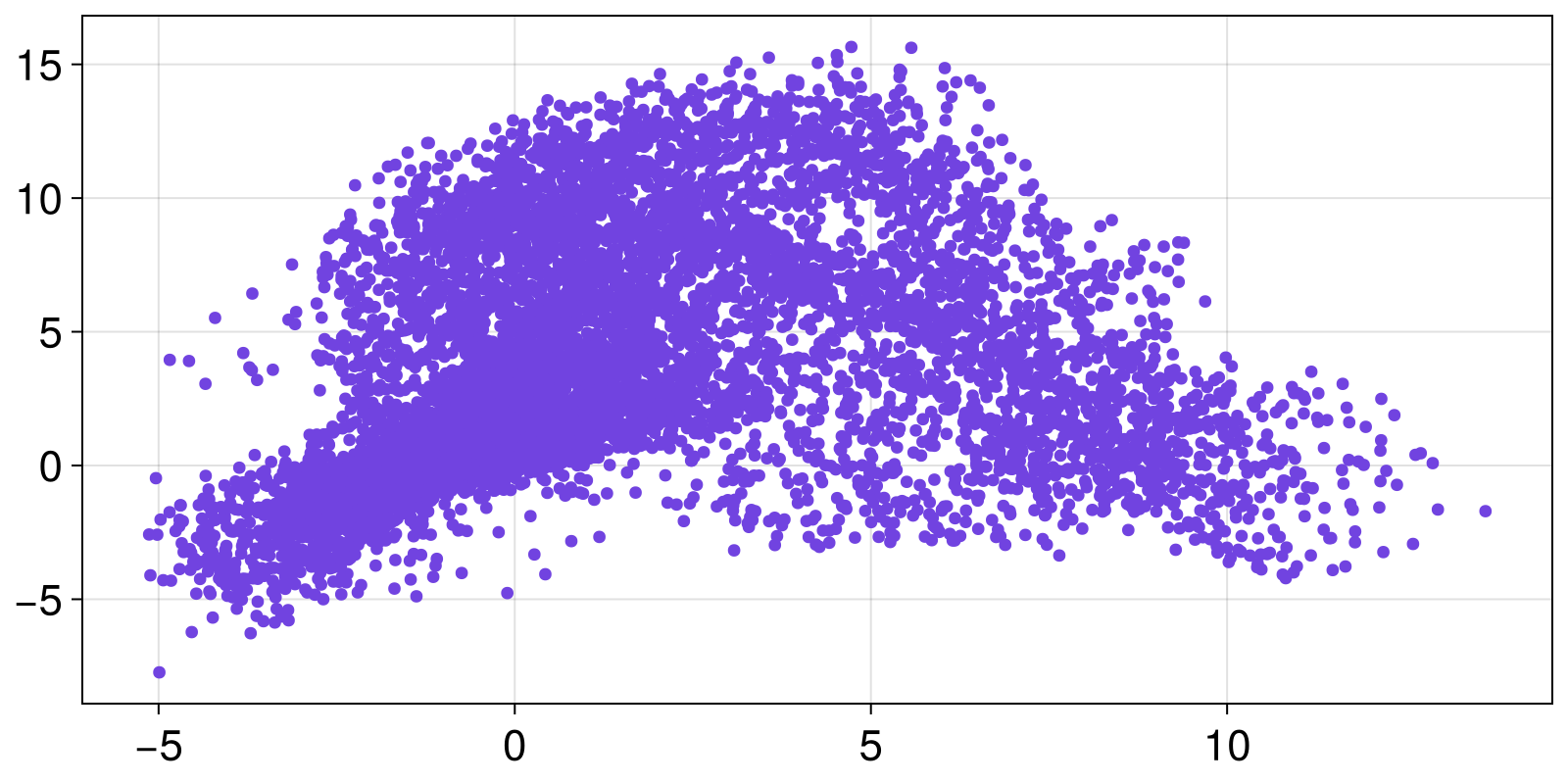
Or, you may want to compute the Lyapunov spectrum of the Lorenz96 system from above, which is a functionality offered by ChaosTools. This is as easy as calling the lyapunovspectrum function with lorenz96
steps = 10_000
lyapunovspectrum(lorenz96, steps)
6-element Vector{Float64}:
1.1829867203063615
0.0007630104170799961
-0.11385364260318617
-0.8267128963288964
-1.5839203337406875
-4.659259733654792As expected, there is at least one positive Lyapunov exponent, because the system is chaotic, and at least one zero Lyapunov exponent, because the system is continuous time.
A fantastic feature of DynamicalSystems.jl is that all library functions work for any applicable dynamical system. The exact same lyapunovspectrum function would also work for the Henon map.
lyapunovspectrum(henon, steps)2-element Vector{Float64}:
0.4167659070649148
-1.6207387113908505Something else that uses a dynamical system is estimating the basins of attraction of a multistable dynamical system. The Henon map is "multistable" in the sense that some initial conditions diverge to infinity, and some others converge to a chaotic attractor. Computing these basins of attraction is simple with Attractors, and would work as follows:
# define a state space grid to compute the basins on:
xg = yg = range(-2, 2; length = 201)
# find attractors using recurrences in state space:
mapper = AttractorsViaRecurrences(henon, (xg, yg); sparse = false)
# compute the full basins of attraction:
basins, attractors = basins_of_attraction(mapper; show_progress = false)
([-1 -1 … -1 -1; -1 -1 … -1 -1; … ; -1 -1 … -1 -1; -1 -1 … -1 -1], Dict{Int64, StateSpaceSet{2, Float64, SVector{2, Float64}}}(1 => 2-dimensional StateSpaceSet{Float64} with 416 points))Let's visualize the result
heatmap_basins_attractors((xg, yg), basins, attractors)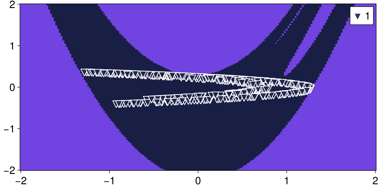
Another component of DynamicalSystems.jl that utilizes a DynamicalSystem instance is PeriodicOrbits, which, you guessed it, finds periodic orbits. In contrast to Attractors, PeriodicOrbits is dediced to finding both stable and unstable periodic orbits. For example, it is known that inside chaotic attractors there resides an infinity of periodic orbits. Let's find many unstable periodic orbits, up to order 8, for the Henon map using an algorithm dedicated to discrete time systems
xs = range(-3.0, 3.0; length = 10)
ys = range(-10.0, 10.0; length = 10)
seeds = [InitialGuess(SVector{2}(x,y), nothing) for x in xs for y in ys]
n = 7
alg = DavidchackLai(n=n, m=6, abstol=1e-7, disttol=1e-10)
output = periodic_orbits(henon, alg, seeds)
output = uniquepos(output)
output = minimal_period.(henon, output) # remove duplicates
17-element Vector{PeriodicOrbit{2, Float64, Int64, Missing}}:
PeriodicOrbit{2, Float64, Int64, Missing}([0.975800051174896, -0.14274001535291814], 2, missing)
PeriodicOrbit{2, Float64, Int64, Missing}([0.48533586255033284, 0.13257298540776663], 6, missing)
PeriodicOrbit{2, Float64, Int64, Missing}([1.0380595354867264, 0.09343569464117174], 6, missing)
PeriodicOrbit{2, Float64, Int64, Missing}([0.5158146929277369, 0.19052591242843564], 7, missing)
PeriodicOrbit{2, Float64, Int64, Missing}([0.14145342273882586, -0.2778519831667656], 7, missing)
PeriodicOrbit{2, Float64, Int64, Missing}([-1.0466775735267917, 0.3549679378175784], 7, missing)
PeriodicOrbit{2, Float64, Int64, Missing}([0.8511588383495811, 0.14270331194999578], 7, missing)
PeriodicOrbit{2, Float64, Int64, Missing}([-1.1313544770895048, -0.3394063431268514], 1, missing)
PeriodicOrbit{2, Float64, Int64, Missing}([0.6313544770895047, 0.18940634312685142], 1, missing)
PeriodicOrbit{2, Float64, Int64, Missing}([-0.3350165883845605, -0.24823626836087187], 8, missing)
PeriodicOrbit{2, Float64, Int64, Missing}([0.32766943484480787, -0.14510659037702986], 8, missing)
PeriodicOrbit{2, Float64, Int64, Missing}([-0.8368082707705344, 0.35013340845532037], 8, missing)
PeriodicOrbit{2, Float64, Int64, Missing}([0.41408979656286904, -0.24263016094884454], 8, missing)
PeriodicOrbit{2, Float64, Int64, Missing}([-0.837141682318264, -0.37761735322708184], 8, missing)
PeriodicOrbit{2, Float64, Int64, Missing}([-0.5230999957229845, 0.32139570874344087], 8, missing)
PeriodicOrbit{2, Float64, Int64, Missing}([-0.7067667772166851, 0.337520980955444], 4, missing)
PeriodicOrbit{2, Float64, Int64, Missing}([-0.44837319092731864, -0.3422356937234222], 8, missing)and now plot them on top of the chaotic attractor that we found in the previous step
A = attractors[1]
fig, ax = scatter(A; color = ("black", 0.5), markersize = 10)
markers = [:rect, :diamond, :utriangle, :dtriangle, :ltriangle, :rtriangle, :pentagon, :hexagon]
cmap = cgrad(:dense, n+1; categorical = true)
for po in output
    scatter!(ax, po.points; markersize=20, color = cmap[po.T], marker=markers[po.T],
    strokewidth = 1, strokecolor = "black")
end
fig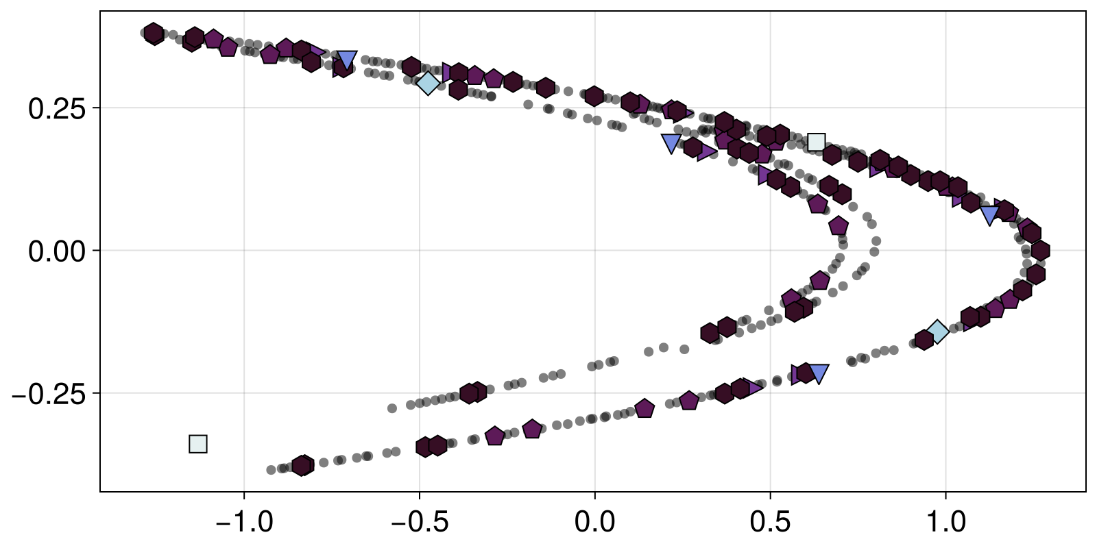
Stochastic systems
DynamicalSystems.jl has some support for stochastic systems in the form of Stochastic Differential Equations (SDEs). Just like CoupledODEs, one can make CoupledSDEs! For example here is a stochastic version of a FitzHugh-Nagumo model
using StochasticDiffEq # load extention for `CoupledSDEs`

function fitzhugh_nagumo(u, p, t)
    x, y = u
    ϵ, β, α, γ, κ, I = p
    dx = (-α * x^3 + γ * x - κ * y + I) / ϵ
    dy = -β * y + x
    return SVector(dx, dy)
end
p = [1.,3.,1.,1.,1.,0.]
sde = CoupledSDEs(fitzhugh_nagumo, zeros(2), p; noise_strength = 0.05)
2-dimensional CoupledSDEs
deterministic: false
discrete time: false
in-place: false
dynamic rule: fitzhugh_nagumo
SDE solver: SOSRA
SDE kwargs: (abstol = 0.01, reltol = 0.01, dt = 0.1)
Noise type: (additive = true, autonomous = true, linear = true, invertible = true)
parameters: [1.0, 3.0, 1.0, 1.0, 1.0, 0.0]
time: 0.0
state: [0.0, 0.0]
In this particular example the SDE noise is white noise (Wiener process) with strength (σ) of 0.05. See the documentation of CoupledSDEs for alternatives.
In any case, in DynamicalSystems.jl all dynamical systems are part of the same interace, stochastic or not. As long as the algorithm is not influenced by stochasticity, we can apply it to CoupledSDEs just as well. For example, we can study multistability in a stochastic system. In contrast to the previous example of the Henon map, we have to use an alternative algorithm, because AttractorsViaRecurrences only works for deterministic systems. So instead we'll use AttractorsViaFeaturizing:
featurizer(X, t) = X[end]

mapper = AttractorsViaFeaturizing(sde, featurizer; Ttr = 200, T = 10)

xg = yg = range(-1, 1; length = 101)

sampler, _ = statespace_sampler((xg, yg))

fs = basins_fractions(mapper, sampler; show_progress = false)
Dict{Int64, Float64} with 2 entries:
2 => 0.508
1 => 0.492and we can see the stored "attractors"
attractors = extract_attractors(mapper)
fig, ax = scatter(attractors[1])
scatter!(attractors[2])
fig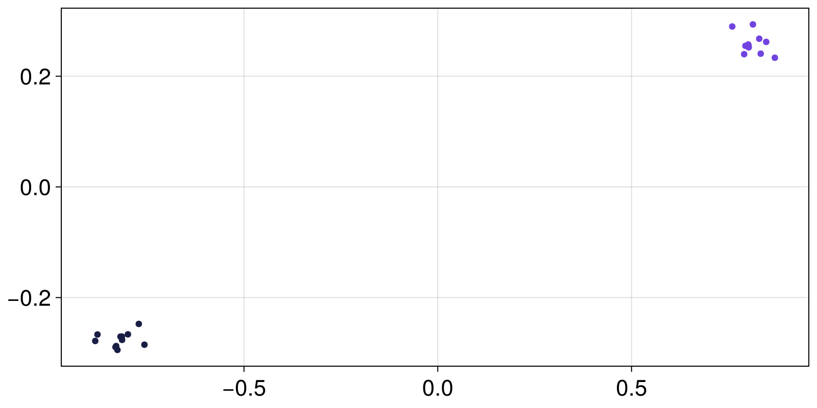
The mathematical concept of attractors doesn't translate trivially to stochastic systems but thankfully this system has two fixed point attractors that are only mildly perturbed by the noise.
Parallelization
Because DynamicalSystems are mutable and most library functions mutate them, one needs to be slightly delicate with parallelization. The package OhMyThreads.jl can take care of all the details for us, like so:
ds = DynamicalSystem(f, u, p) # some concrete implementation
parameters = 0:0.01:1
outputs = zeros(length(parameters))

using OhMyThreads: @tasks, @local
@tasks for i in eachindex(parameters)
    @local system = deepcopy(ds) # important!
    set_parameter!(system, 1, parameters[i])
    outputs[i] = expesive_function(system, args...)
end
Note that parallelization is only useful if the expensive function is significantly more expensive than copying the system and thread communication!
Interactive GUIs
A particularly useful feature are interactive GUI apps one can launch to examine a DynamicalSystem. The simplest is interactive_trajectory_timeseries. To actually make it interactive one needs to enable GLMakie.jl as a backend:
import GLMakie
GLMakie.activate!()
and then launch the app:
u0s = [10rand(5) for _ in 1:3]
parameter_sliders = Dict(1 => 0:0.01:32)

fig, dsobs = interactive_trajectory_timeseries(
    lorenz96, [1, 2, 3, 4, 5], u0s;
    Δt = 0.02, parameter_sliders
)
fig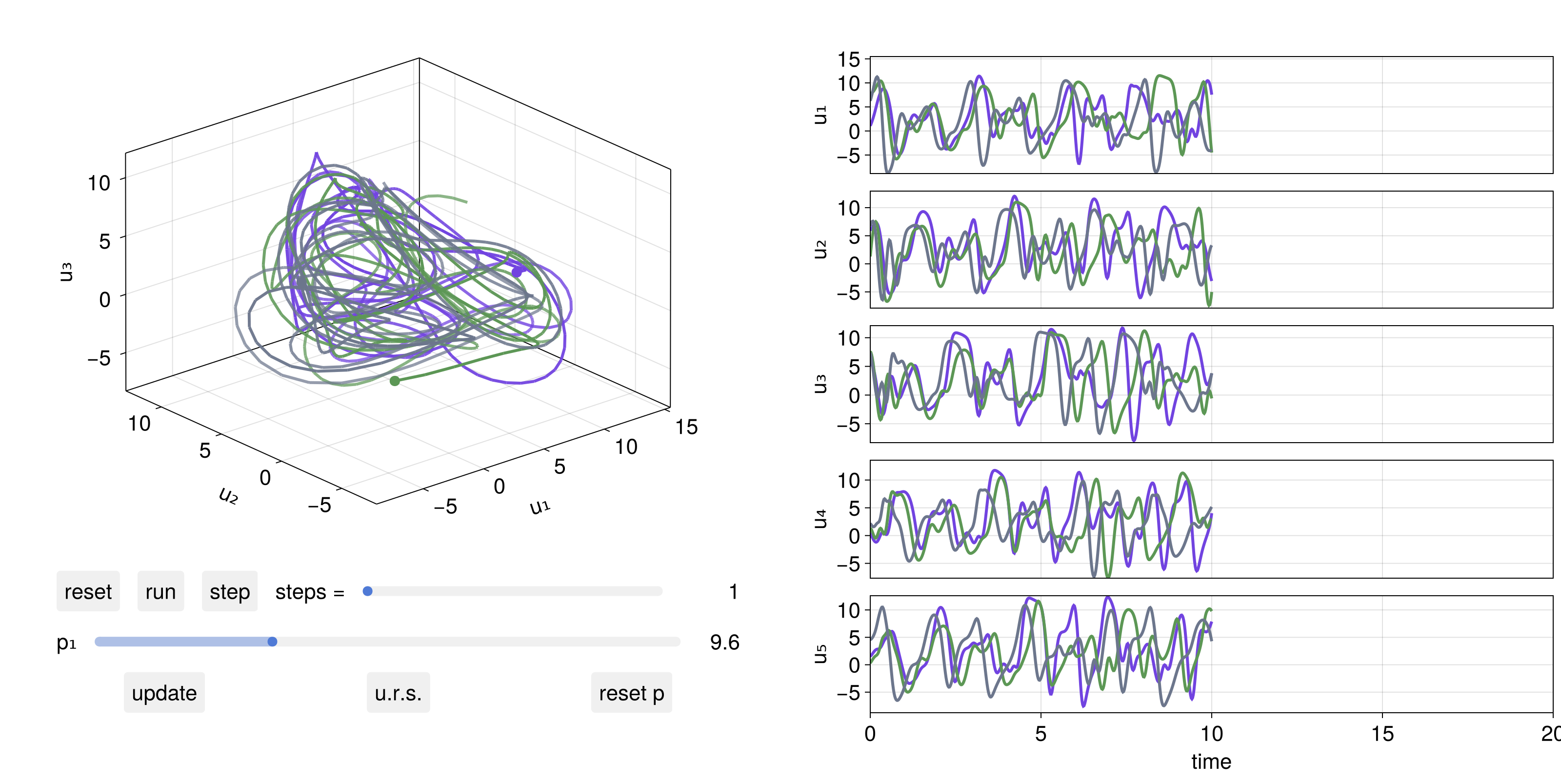
Developing new algorithms
You could also be using a DynamicalSystem instance directly to build your own algorithm if it isn't already implemented (and then later contribute it so it is implemented ;) ). A dynamical system can be evolved forwards in time using step!:
henon2-dimensional DeterministicIteratedMap
deterministic: true
discrete time: true
in-place: false
dynamic rule: henon_rule
parameters: [1.4, 0.3]
time: 4
state: [0.8645652364614893, 0.1468830114550427]
Notice how the time is not 0, because henon has already been stepped when we called the function basins_of_attraction with it. We can step it more:
step!(henon)2-dimensional DeterministicIteratedMap
deterministic: true
discrete time: true
in-place: false
dynamic rule: henon_rule
parameters: [1.4, 0.3]
time: 5
state: [0.10042074411824756, 0.25936957093844676]
step!(henon, 2)2-dimensional DeterministicIteratedMap
deterministic: true
discrete time: true
in-place: false
dynamic rule: henon_rule
parameters: [1.4, 0.3]
time: 7
state: [-1.1407856457447472, 0.37357545442484374]
For more information on how to directly use DynamicalSystem instances, see the interface of DynamicalSystem.
State space sets
Let's recall that the output of the trajectory function is a StateSpaceSet:
X2-dimensional StateSpaceSet{Float64} with 10001 points
0.2 0.3
1.244 0.06
-1.10655 0.3732
-0.341035 -0.331965
0.505208 -0.102311
0.540361 0.151562
0.742777 0.162108
0.389703 0.222833
1.01022 0.116911
-0.311842 0.303065
⋮
-0.582534 0.328346
0.853262 -0.17476
-0.194038 0.255978
1.20327 -0.0582113
-1.08521 0.36098
-0.287758 -0.325562
0.558512 -0.0863275
0.476963 0.167554
0.849062 0.143089This is the main data structure used in DynamicalSystems.jl to handle numerical data. It is printed like a matrix where each column is the timeseries of each dynamic variable. In reality, it is a vector equally-sized vectors representing state space points. (For advanced users: StateSpaceSet directly subtypes AbstractVector{<:AbstractVector})
When indexed with 1 index, it behaves like a vector of vectors
X[1]2-element SVector{2, Float64} with indices SOneTo(2):
0.2
0.3X[2:5]2-dimensional StateSpaceSet{Float64} with 4 points
1.244 0.06
-1.10655 0.3732
-0.341035 -0.331965
0.505208 -0.102311When indexed with two indices, it behaves like a matrix
X[7:13, 2] # 2nd column7-element Vector{Float64}:
0.1621081681101694
0.22283309461548204
0.11691103950545975
0.30306503631282444
-0.09355263057973214
0.35007640234803744
-0.29998206408499634When iterated, it iterates over the contained points
for (i, point) in enumerate(X)
    @show point
    i > 5 && break
end
point = [0.2, 0.3]
point = [1.244, 0.06]
point = [-1.1065503999999997, 0.3732]
point = [-0.34103530283622296, -0.3319651199999999]
point = [0.5052077711071681, -0.10231059085086688]
point = [0.5403605603672313, 0.1515623313321504]map(point -> point[1] + 1/(point[2]+0.1), X)10001-element Vector{Float64}:
2.7
7.494
1.006720944040575
-4.652028265916192
-432.28452634595817
4.515518505137784
4.557995741581754
3.4872793228808314
5.620401692451571
2.1691470931310732
⋮
1.752024323892008
-12.522817477226136
2.6151207744662046
25.133206775921803
1.0840850677362275
-4.721137673509619
73.69787164232238
4.214533120554577
4.9627832739756785The columns of the set are obtained with the convenience columns function
x, y = columns(X)
summary.((x, y))
("10001-element Vector{Float64}", "10001-element Vector{Float64}")Because StateSpaceSet really is a vector of vectors, it can be given to any Julia function that accepts such an input. For example, the Makie plotting ecosystem knows how to plot vectors of vectors. That's why this works:
scatter(X)
even though Makie has no knowledge of the specifics of StateSpaceSet.
Nonlinear data anlysis using state space sets
Several packages of the library deal with StateSpaceSets.
You could use ComplexityMeasures to obtain the entropy, or other complexity measures, of a given set. Below, we obtain the entropy of the natural density of the chaotic attractor by partitioning into a histogram of approximately 50 bins per dimension:
prob_est = ValueHistogram(50)
entropy(prob_est, X)7.825799208736613Or, obtain the permutation and sample entropies of the two columns of X:
pex = entropy_permutation(x; m = 4)
sey = entropy_sample(y; m = 2)
pex, sey
(3.15987571159201, 0.02579132263914716)Alternatively, you could use FractalDimensions to get the fractal dimensions of the chaotic attractor of the henon map using the Grassberger-Procaccia algorithm:
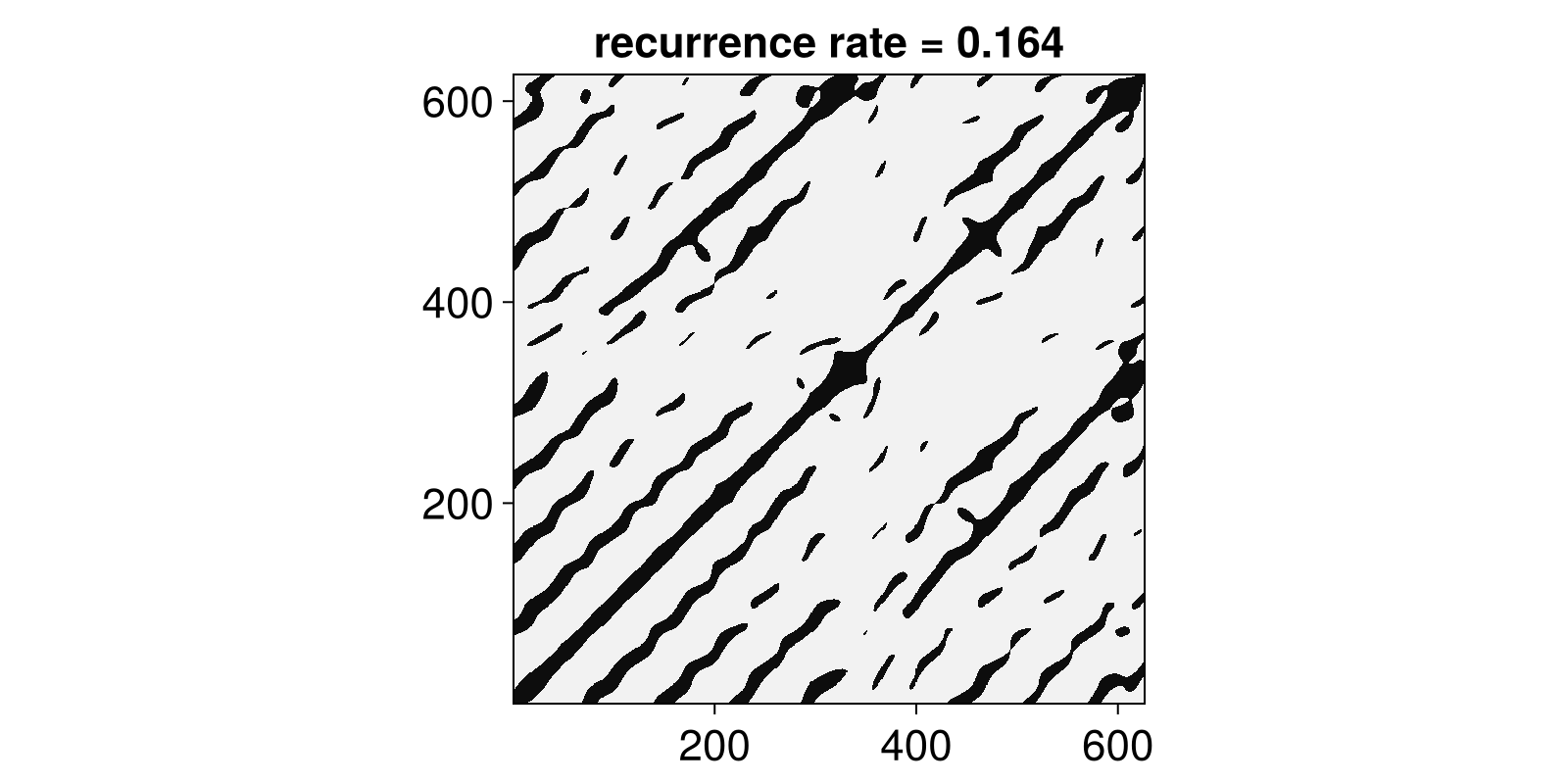
grassberger_proccacia_dim(X; show_progress = false)1.2232922815092426Or, you could obtain a recurrence matrix of a state space set with RecurrenceAnalysis
R = RecurrenceMatrix(Y, 8.0)
Rg = grayscale(R)
rr = recurrencerate(R)
heatmap(Rg; colormap = :grays,
    axis = (title = "recurrence rate = $(round(rr; digits = 3))", aspect = 1)
)
More nonlinear timeseries analysis
A trajectory of a known dynamical system is one way to obtain a StateSpaceSet. However, another common way is via a delay coordinates embedding of a measured/observed timeseries. For example, we could use optimal_separated_de from DelayEmbeddings to create an optimized delay coordinates embedding of a timeseries
w = Y[:, 1] # first variable of Lorenz96
𝒟, τ, e = optimal_separated_de(w)
𝒟
5-dimensional StateSpaceSet{Float64} with 558 points
3.15369 -2.40036 1.60497 2.90499 5.72572
2.71384 -2.24811 1.55832 3.04987 5.6022
2.2509 -2.02902 1.50499 3.20633 5.38629
1.77073 -1.75077 1.45921 3.37699 5.07029
1.27986 -1.42354 1.43338 3.56316 4.65003
0.785468 -1.05974 1.43672 3.76473 4.12617
0.295399 -0.673567 1.47423 3.98019 3.50532
-0.181891 -0.280351 1.54635 4.20677 2.80048
-0.637447 0.104361 1.64932 4.44054 2.03084
-1.06201 0.465767 1.77622 4.67654 1.22067
⋮
7.42111 9.27879 -1.23936 5.15945 3.25618
7.94615 9.22663 -1.64222 5.24344 3.34749
8.40503 9.13776 -1.81947 5.26339 3.46932
8.78703 8.99491 -1.77254 5.22631 3.60343
9.08701 8.77963 -1.51823 5.13887 3.72926
9.30562 8.47357 -1.08603 5.00759 3.82705
9.4488 8.06029 -0.514333 4.83928 3.88137
9.52679 7.52731 0.153637 4.6414 3.88458
9.55278 6.86845 0.873855 4.42248 3.83902and compare
fig = Figure()
axs = [Axis3(fig[1, i]) for i in 1:2]
for (S, ax) in zip((Y, 𝒟), axs)
    lines!(ax, S[:, 1], S[:, 2], S[:, 3])
end
fig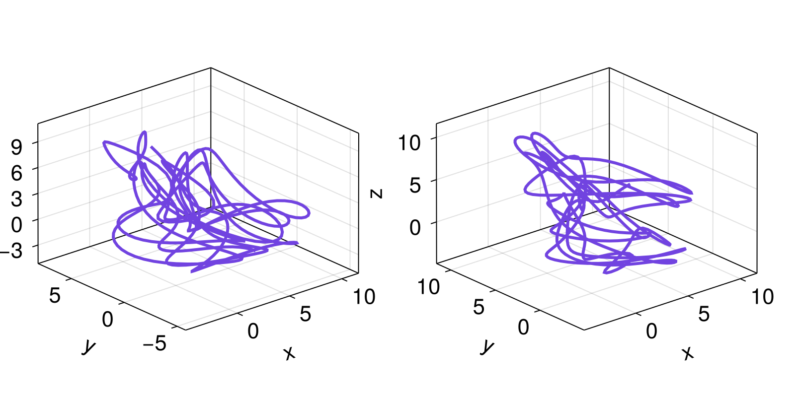
Since 𝒟 is just another state space set, we could be using any of the above analysis pipelines on it just as easily.
TimeseriesSurrogates ties well all other observed/measured data analysis by providing a framework for hypothesis testing. For example, if we had a measured timeseries but we were not sure whether it represents a deterministic system with structure in the state space, or mostly noise, we could do a surrogate test. Let's say that this is the timeseries we want to use:
x # Henon map timeseries
# contaminate with noise
using Random: Xoshiro
rng = Xoshiro(1234)
noisyx = x .+ randn(rng, length(x))/100
10001-element Vector{Float64}:
0.20970656328855217
1.234207815884648
-1.0975317911640587
-0.34136333412866937
0.49919984887361246
0.525908789214369
0.7698512214687646
0.40494794365255515
1.0178148279094894
-0.32065647099440525
⋮
-0.5795026223156395
0.8506112680355368
-0.19401795429457597
1.1986459649969237
-1.0820164160511792
-0.281009566309449
0.565898869505943
0.47369878723368636
0.847005938798569To do the test, we use SurrogateTest and RandomFourier from TimeseriesSurrogates. We need to provide a function that given a timeseries it outputs a discriminatory value, which is typically some nonlinear measure. Here we will use the generalized_dim from FractalDimensions (because it performs better in noisy sets) applied to the delay embedded set of the timeseries.
discriminatory(x) = generalized_dim(embed(x, 2, 1); show_progress = false)discriminatory (generic function with 1 method)we then initialize the test and obtain its p-value:
surrogate_method = RandomFourier()
test = SurrogateTest(discriminatory, noisyx, surrogate_method; n = 1000)
pval = pvalue(test)0.0Since the p-value is very small we have good confidence that the timeseries come from some nonlinear system and they are not just noise.
The last component of DynamicalSystems.jl to mention is SignalDecomposition, a general-purpose tool that can perform de-noising or de-trending in timeseries, a step often useful when pre-processing data before further analysis. It incorporates several linear and nonlinear techniques. For example, one can attempt to de-noise the noisy Henon map timeseries we used above with nonlinear techniques, for example:
m = 5
k = 15
Q = [3, 3, 3, 3, 3]
denoisedx, _ = SignalDecomposition.decompose(noisyx, ManifoldProjection(m, Q, k))
fig, ax = lines(abs.(x .- noisyx); label = "noise error")
lines!(ax, abs.(x .- denoisedx); label = "denoised error")
ylims!(ax, 0, 0.05)
axislegend(ax)
fig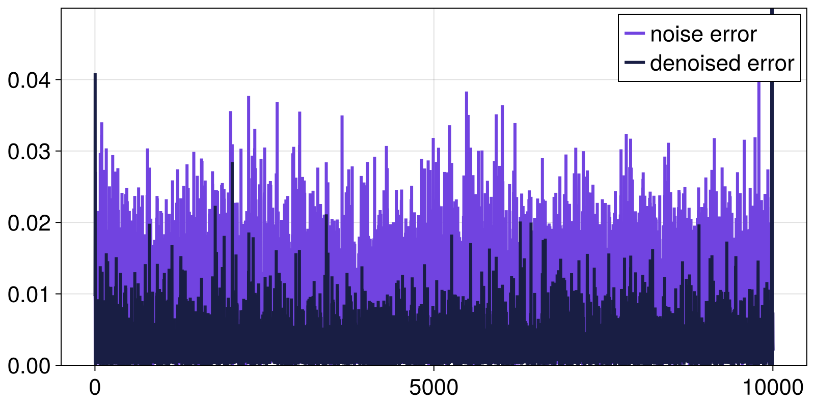
Integration with ModelingToolkit.jl
DynamicalSystems.jl understands when a model has been generated via ModelingToolkit.jl. The symbolic variables used in ModelingToolkit.jl can be used to access the state or parameters of the dynamical system.
To access this functionality, the DynamicalSystem must be created from a DEProblem of the SciML ecosystem, and the DEProblem itself must be created from a ModelingToolkit.jl model.
ProcessBasedModelling.jl is an extension to ModelingToolkit.jl for creating models from a set of equations. It has been designed to be useful for scenarios applicable to a typical nonlinear dynamics analysis workflow, and provides improved error messages during system construction versus MTK. Have a look at its docs!
Let's create a the Roessler system as an MTK model:
using ModelingToolkit

@variables t # use unitless time
D = Differential(t)
@mtkmodel Roessler begin
    @parameters begin
        a = 0.2
        b = 0.2
        c = 5.7
    end
    @variables begin
        x(t) = 1.0
        y(t) = 0.0
        z(t) = 0.0
        nlt(t) # nonlinear term
    end
    @equations begin
        D(x) ~ -y -z
        D(y) ~ x + a*y
        D(z) ~ b + nlt
        nlt ~ z*(x - c)
    end
end

@mtkcompile model = Roessler()
\[ \begin{align} \frac{\mathrm{d} z\left( t \right)}{\mathrm{d}t} &= b + \mathtt{nlt}\left( t \right) \\ \frac{\mathrm{d} y\left( t \right)}{\mathrm{d}t} &= x\left( t \right) + a y\left( t \right) \\ \frac{\mathrm{d} x\left( t \right)}{\mathrm{d}t} &= - y\left( t \right) - z\left( t \right) \end{align} \]
this model can then be made into an ODEProblem.
prob = ODEProblem(model, nothing, (0.0, Inf))ODEProblem with uType Vector{Float64} and tType Float64. In-place: true
Initialization status: FULLY_DETERMINED
Non-trivial mass matrix: false
timespan: (0.0, Inf)
u0: 3-element Vector{Float64}:
0.0
0.0
1.0We used nothing for the initialization container as all parameters and state variables have been created with default values.
Now, this problem can be made into a CoupledODEs:
roessler = CoupledODEs(prob)3-dimensional CoupledODEs
deterministic: true
discrete time: false
in-place: true
dynamic rule: GeneratedFunctionWrapper
ODE solver: Tsit5
ODE kwargs: (abstol = 1.0e-6, reltol = 1.0e-6)
parameters: ModelingToolkit.MTKParameters{Vector{Float64}, Vector{Float64}, Tuple{}, Tuple{}, Tuple{}, Tuple{}}([0.2, 0.2, 5.7], [0.0, 0.0, 1.0, 0.0, 0.0, 0.0, 0.0, 0.0], (), (), (), ())
time: 0.0
state: [0.0, 0.0, 1.0]
This dynamical system instance can be used in the rest of the library like anything else. Additionally, you can "observe" referenced symbolic variables:
observe_state(roessler, model.x)1.0or, more commonly, you can observe a Symbol that has the name of the symbolic variable:
observe_state(roessler, :nlt)-0.0These observables can also be used in the GUI visualization interactive_trajectory_timeseries.
You can also symbolically query or alter parameters
current_parameter(roessler, :c)5.7set_parameter!(roessler, :c, 5.0)current_parameter(roessler, :c)5.0This symbolic indexing can be given anywhere in the ecosystem where you would be altering the parameters, such as the function global_continuation from Attractors.
Core components reference
StateSpaceSets.StateSpaceSet — Type
StateSpaceSet{D, T, V} <: AbstractVector{V}A dedicated interface for sets in a state space. It is an ordered container of equally-sized points of length D, with element type T, represented by a vector of type V. Typically V is SVector{D,T} or Vector{T} and the data are always stored internally as Vector{V}. SSSet is an alias for StateSpaceSet.
The underlying Vector{V} can be obtained by vec(ssset), although this is almost never necessary because StateSpaceSet subtypes AbstractVector and extends its interface. StateSpaceSet also supports almost all sensible vector operations like append!, push!, hcat, eachrow, among others. When iterated over, it iterates over its contained points.
Construction
Constructing a StateSpaceSet is done in three ways:
- By giving in each individual columns of the state space set as
Vector{<:Real}:StateSpaceSet(x, y, z, ...). - By giving in a matrix whose rows are the state space points:
StateSpaceSet(m). - By giving in directly a vector of vectors (state space points):
StateSpaceSet(v_of_v).
All constructors allow for two keywords:
containerwhich sets the type ofV(the type of inner vectors). At the moment options are onlySVector,MVector, orVector, and by defaultSVectoris used.nameswhich can be an iterable of lengthDwhose elements areSymbols. This allows assigning a name to each dimension and accessing the dimension by name, see below.namesisnothingif not given. UseStateSpaceSet(s; names)to add names to an existing sets.
Description of indexing
When indexed with 1 index, StateSpaceSet behaves exactly like its encapsulated vector. i.e., a vector of vectors (state space points). When indexed with 2 indices it behaves like a matrix where each row is a point.
In the following let i, j be integers, typeof(X) <: AbstractStateSpaceSet and v1, v2 be <: AbstractVector{Int} (v1, v2 could also be ranges, and for performance benefits make v2 an SVector{Int}).
X[i] == X[i, :]gives theith point (returns anSVector)X[v1] == X[v1, :], returns aStateSpaceSetwith the points in those indices.X[:, j]gives thejth variable timeseries (or collection), asVectorX[v1, v2], X[:, v2]returns aStateSpaceSetwith the appropriate entries (first indices being "time"/point index, while second being variables)X[i, j]value of thejth variable, at theith timepoint
In all examples above, j can also be a Symbol, provided that names has been given when creating the state space set. This allows accessing a dimension by name. This is provided as a convenience and it is not an optimized operation, hence recommended to be used primarily with X[:, j::Symbol].
Use Matrix(ssset) or StateSpaceSet(matrix) to convert. It is assumed that each column of the matrix is one variable. If you have various timeseries vectors x, y, z, ... pass them like StateSpaceSet(x, y, z, ...). You can use columns(dataset) to obtain the reverse, i.e. all columns of the dataset in a tuple.
DynamicalSystemsBase.DynamicalSystem — Type
DynamicalSystemDynamicalSystem is an abstract supertype encompassing all concrete implementations of what counts as a "dynamical system" in the DynamicalSystems.jl library.
All concrete implementations of DynamicalSystem can be iteratively evolved in time via the step! function. Hence, most library functions that evolve the system will mutate its current state and/or parameters. See the documentation online for implications this has for parallelization.
DynamicalSystem is further separated into two abstract types: ContinuousTimeDynamicalSystem, DiscreteTimeDynamicalSystem. The simplest and most common concrete implementations of a DynamicalSystem are DeterministicIteratedMap or CoupledODEs.
Description
A DynamicalSystem represents the time evolution of a state in a state space. It mainly encapsulates three things:
- A state, typically referred to as
u, with initial valueu0. The space thatuoccupies is the state space ofdsand the length ofuis the dimension ofds(and of the state space). - A dynamic rule, typically referred to as
f, that dictates how the state evolves/changes with time when calling thestep!function.fis typically a standard Julia function, see the online documentation for examples. - A parameter container
pthat parameterizesf.pcan be anything, but in general it is recommended to be a type-stable mutable container.
In sort, any set of quantities that change in time can be considered a dynamical system, however the concrete subtypes of DynamicalSystem are much more specific in their scope. Concrete subtypes typically also contain more information than the above 3 items.
In this scope dynamical systems have a known dynamic rule f. Finite measured or sampled data from a dynamical system are represented using StateSpaceSet. Such data are obtained from the trajectory function or from an experimental measurement of a dynamical system with an unknown dynamic rule.
See also the DynamicalSystems.jl tutorial online for examples making dynamical systems.
Integration with ModelingToolkit.jl (MTK)
Dynamical systems that have been constructed from DEProblems that themselves have been constructed from ModelingToolkit.jl keep a reference to the symbolic model and all symbolic variables. Accessing a DynamicalSystem using symbolic variables is possible via the functions observe_state, set_state!, current_parameter and set_parameter!. The referenced MTK model corresponding to the dynamical system can be obtained with model = referrenced_sciml_model(ds::DynamicalSystem).
See also the DynamicalSystems.jl tutorial online for an example.
ModelingToolkit.jl treats initial conditions of all variables as additional parameters. This is because its terminology is aimed primarily at initial value problems rather than dynamical systems. It is strongly recommended when making a dynamical system from an MTK model to only access parameters via symbols, and to not use the split = false keyword when creating the problem type from the MTK model.
API
The API that DynamicalSystem employs is composed of the functions listed below. Once a concrete instance of a subtype of DynamicalSystem is obtained, it can queried or altered with the following functions.
The main use of a concrete dynamical system instance is to provide it to downstream functions such as lyapunovspectrum from ChaosTools.jl or basins_of_attraction from Attractors.jl. A typical user will likely not utilize directly the following API, unless when developing new algorithm implementations that use dynamical systems.
API - obtain information
ds(t)withdsan instance ofDynamicalSystem: return the state ofdsat timet. For continuous time systems this interpolates current and previous time step and is very accurate; for discrete time systems it only works iftis the current time.current_stateinitial_stateobserve_statecurrent_parameterscurrent_parameterinitial_parametersisdeterministicisdiscretetimedynamic_rulecurrent_timeinitial_timeisinplacesuccessful_stepreferrenced_sciml_modelnamed_variables
API - alter status
Dynamical system implementations
DynamicalSystemsBase.DeterministicIteratedMap — Type
DeterministicIteratedMap <: DiscreteTimeDynamicalSystem
DeterministicIteratedMap(f, u0, p = nothing; t0 = 0)
A deterministic discrete time dynamical system defined by an iterated map as follows:
\[\vec{u}_{n+1} = \vec{f}(\vec{u}_n, p, n)\]
An alias for DeterministicIteratedMap is DiscreteDynamicalSystem.
Optionally configure the parameter container p and initial time t0.
For construction instructions regarding f, u0 see the DynamicalSystems.jl tutorial.
DynamicalSystemsBase.CoupledODEs — Type
CoupledODEs <: ContinuousTimeDynamicalSystem
CoupledODEs(f, u0 [, p]; diffeq, t0 = 0.0)
A deterministic continuous time dynamical system defined by a set of coupled ordinary differential equations as follows:
\[\frac{d\vec{u}}{dt} = \vec{f}(\vec{u}, p, t)\]
An alias for CoupledODE is ContinuousDynamicalSystem.
Optionally provide the parameter container p and initial time as keyword t0.
For construction instructions regarding f, u0 see the DynamicalSystems.jl tutorial.
DifferentialEquations.jl interfacing
The ODEs are evolved via the solvers of DifferentialEquations.jl. When initializing a CoupledODEs, you can specify the solver that will integrate f in time, along with any other integration options, using the diffeq keyword. For example you could use diffeq = (abstol = 1e-9, reltol = 1e-9). If you want to specify a solver, do so by using the keyword alg, e.g.: diffeq = (alg = Tsit5(), reltol = 1e-6). This requires you to have been first using OrdinaryDiffEq (or smaller library package such as OrdinaryDiffEqVerner) to access the solvers. The default diffeq is:
(alg = OrdinaryDiffEqTsit5.Tsit5{typeof(OrdinaryDiffEqCore.triviallimiter!), typeof(OrdinaryDiffEqCore.triviallimiter!), Static.False}(OrdinaryDiffEqCore.triviallimiter!, OrdinaryDiffEqCore.triviallimiter!, static(false)), abstol = 1.0e-6, reltol = 1.0e-6)
diffeq keywords can also include callback for event handling .
The convenience constructors CoupledODEs(prob::ODEProblem [, diffeq]) and CoupledODEs(ds::CoupledODEs [, diffeq]) are also available. Use ODEProblem(ds::CoupledODEs, tspan = (t0, Inf)) to obtain the problem.
To integrate with ModelingToolkit.jl, the dynamical system must be created via the ODEProblem (which itself is created via ModelingToolkit.jl), see the Tutorial for an example.
Dev note: CoupledODEs is a light wrapper of ODEIntegrator from DifferentialEquations.jl.
DynamicalSystemsBase.StroboscopicMap — Type
StroboscopicMap <: DiscreteTimeDynamicalSystem
StroboscopicMap(ds::CoupledODEs, period::Real) → smap
StroboscopicMap(period::Real, f, u0, p = nothing; kwargs...)
A discrete time dynamical system that produces iterations of a time-dependent (non-autonomous) CoupledODEs system exactly over a given period. The second signature first creates a CoupledODEs and then calls the first.
StroboscopicMap follows the DynamicalSystem interface. In addition, the function set_period!(smap, period) is provided, that sets the period of the system to a new value (as if it was a parameter). As this system is in discrete time, current_time and initial_time are integers. The initial time is always 0, because current_time counts elapsed periods. Call these functions on the parent of StroboscopicMap to obtain the corresponding continuous time. In contrast, reinit! expects t0 in continuous time.
The convenience constructor
StroboscopicMap(T::Real, f, u0, p = nothing; diffeq, t0 = 0) → smapis also provided.
See also PoincareMap.
DynamicalSystemsBase.PoincareMap — Type
PoincareMap <: DiscreteTimeDynamicalSystem
PoincareMap(ds::CoupledODEs, plane; kwargs...) → pmap
A discrete time dynamical system that produces iterations over the Poincaré map[DatserisParlitz2022] of the given continuous time ds. This map is defined as the sequence of points on the Poincaré surface of section, which is defined by the plane argument.
Iterating pmap also mutates ds which is referrenced in pmap.
See also StroboscopicMap, poincaresos.
Keyword arguments
direction = -1: Only crossings withsign(direction)are considered to belong to the surface of section. Negative direction means going from less than $b$ to greater than $b$.u0 = nothing: Specify an initial state. Ifnothingit is thecurrent_state(ds).rootkw = (xrtol = 1e-6, atol = 1e-8): ANamedTupleof keyword arguments passed tofind_zerofrom Roots.jl.Tmax = 1e3: The argumentTmaxexists so that the integrator can terminate instead of being evolved for infinite time, to avoid cases where iteration would continue forever for ill-defined hyperplanes or for convergence to fixed points, where the trajectory would never cross again the hyperplane. If during onestep!the system has been evolved for more thanTmax, thenstep!(pmap)will terminate and error.
Description
The Poincaré surface of section is defined as sequential transversal crossings a trajectory has with any arbitrary manifold, but here the manifold must be a hyperplane. PoincareMap iterates over the crossings of the section.
If the state of ds is $\mathbf{u} = (u_1, \ldots, u_D)$ then the equation defining a hyperplane is
\[a_1u_1 + \dots + a_Du_D = \mathbf{a}\cdot\mathbf{u}=b\]
where $\mathbf{a}, b$ are the parameters of the hyperplane.
In code, plane can be either:
- A
Tuple{Int, <: Real}, like(j, r): the plane is defined as when thejth variable of the system equals the valuer. - A vector of length
D+1. The firstDelements of the vector correspond to $\mathbf{a}$ while the last element is $b$.
PoincareMap uses ds, higher order interpolation from DifferentialEquations.jl, and root finding from Roots.jl, to create a high accuracy estimate of the section.
PoincareMap follows the DynamicalSystem interface with the following adjustments:
dimension(pmap) == dimension(ds), even though the Poincaré map is effectively 1 dimension less.- Like
StroboscopicMaptime is discrete and counts the iterations on the surface of section.initial_timeis always0andcurrent_timeis current iteration number. - A new function
current_crossing_timereturns the real time corresponding to the latest crossing of the hyperplane. The corresponding state on the hyperplane iscurrent_state(pmap)as expected. - For the special case of
planebeing aTuple{Int, <:Real}, a specialreinit!method is allowed with input state of lengthD-1instead ofD, i.e., a reduced state already on the hyperplane that is then converted into theDdimensional state. - The
initial_state(pmap)returns the state initial state of the map. This is notu0becauseu0is evolved forwards until it resides on the Poincaré plane. - In the
reinit!function, thet0keyword denotes the starting time of the continuous time dynamical system, as the starting time of thePoincareMapis by definition always 0.
Example
using DynamicalSystemsBase, PredefinedDynamicalSystems
ds = Systems.rikitake(zeros(3); μ = 0.47, α = 1.0)
pmap = poincaremap(ds, (3, 0.0))
step!(pmap)
next_state_on_psos = current_state(pmap)DynamicalSystemsBase.ProjectedDynamicalSystem — Type
ProjectedDynamicalSystem <: DynamicalSystem
ProjectedDynamicalSystem(ds::DynamicalSystem, projection, complete_state)
A dynamical system that represents a projection of an existing ds on a (projected) space.
The projection defines the projected space. If projection isa AbstractVector{Int}, then the projected space is simply the variable indices that projection contains. Otherwise, projection can be an arbitrary function that given the state of the original system ds, returns the state in the projected space. In this case the projected space can be equal, or even higher-dimensional, than the original.
complete_state produces the state for the original system from the projected state. complete_state can always be a function that given the projected state returns a state in the original space. However, if projection isa AbstractVector{Int}, then complete_state can also be a vector that contains the values of the remaining variables of the system, i.e., those not contained in the projected space. In this case the projected space needs to be lower-dimensional than the original.
Notice that ProjectedDynamicalSystem does not require an invertible projection, complete_state is only used during reinit!. ProjectedDynamicalSystem is in fact a rather trivial wrapper of ds which steps it as normal in the original state space and only projects as a last step, e.g., during current_state.
Examples
Case 1: project 5-dimensional system to its last two dimensions.
ds = Systems.lorenz96(5)
projection = [4, 5]
complete_state = [0.0, 0.0, 0.0] # completed state just in the plane of last two dimensions
prods = ProjectedDynamicalSystem(ds, projection, complete_state)
reinit!(prods, [0.2, 0.4])
step!(prods)
current_state(prods)
Case 2: custom projection to general functions of state.
ds = Systems.lorenz96(5)
projection(u) = [sum(u), sqrt(u[1]^2 + u[2]^2)]
complete_state(y) = repeat([y[1]/5], 5)
prods = # same as in above example...DynamicalSystemsBase.ArbitrarySteppable — Type
ArbitrarySteppable <: DiscreteTimeDynamicalSystem
ArbitrarySteppable(
    model, step!, extract_state, extract_parameters, reset_model!;
    isdeterministic = true, set_state = reinit!,
)
A dynamical system generated by an arbitrary "model" that can be stepped in-place with some function step!(model) for 1 step. The state of the model is extracted by the extract_state(model) -> u function The parameters of the model are extracted by the extract_parameters(model) -> p function. The system may be re-initialized, via reinit!, with the reset_model! user-provided function that must have the call signature
reset_model!(model, u, p)given a (potentially new) state u and parameter container p, both of which will default to the initial ones in the reinit! call.
ArbitrarySteppable exists to provide the DynamicalSystems.jl interface to models from other packages that could be used within the DynamicalSystems.jl library. ArbitrarySteppable follows the DynamicalSystem interface with the following adjustments:
initial_timeis always 0, as time counts the steps the model has taken since creation or lastreinit!call.set_state!is the same asreinit!by default. If not, the keyword argumentset_stateis a functionset_state(model, u)that sets the state of the model tou.- The keyword
isdeterministicshould be set properly, as it decides whether downstream algorithms should error or not.
DynamicalSystemsBase.CoupledSDEs — Type
CoupledSDEs <: ContinuousTimeDynamicalSystem
CoupledSDEs(f, u0 [, p]; kwargs...)
A stochastic continuous time dynamical system defined by a set of coupled stochastic differential equations (SDEs) as follows:
\[\text{d}\mathbf{u} = \mathbf{f}(\mathbf{u}, p, t) \text{d}t + \mathbf{g}(\mathbf{u}, p, t) \text{d}\mathcal{N}_t\]
where $\mathbf{u}(t)$ is the state vector at time $t$, $\mathbf{f}$ describes the deterministic dynamics, and the noise term $\mathbf{g}(\mathbf{u}, p, t) \text{d}\mathcal{N}_t$ describes the stochastic forcing in terms of a noise function (or diffusion function) $\mathbf{g}$ and a noise process $\mathcal{N}_t$. The parameters of the functions $\mathcal{f}$ and $\mathcal{g}$ are contained in the vector $p$.
There are multiple ways to construct a CoupledSDEs depending on the type of stochastic forcing.
The only required positional arguments are the deterministic dynamic rule f(u, p, t), the initial state u0, and optinally the parameter container p (by default p = nothing). For construction instructions regarding f, u0 see the DynamicalSystems.jl tutorial .
By default, the noise term is standard Brownian motion, i.e. additive Gaussian white noise with identity covariance matrix. To construct different noise structures, see below.
Noise term
The noise term can be specified via several keyword arguments. Based on these keyword arguments, the noise function g is constructed behind the scenes unless explicitly given.
- The noise strength (i.e. the magnitude of the stochastic forcing) can be scaled with
noise_strength(defaults to1.0). This factor is multiplied with the whole noise term. - For non-diagonal and correlated noise, a covariance matrix can be provided via
covariance(defaults to identity matrix of sizelength(u0).) - For more complicated noise structures, including state- and time-dependent noise, the noise function
gcan be provided explicitly as a keyword argument (defaults tonothing). For construction instructions, continue reading.
The function g interfaces to the diffusion function specified in an SDEProblem of DynamicalSystems.jl. g must follow the same syntax as f, i.e., g(u, p, t) for out-of-place (oop) and g!(du, u, p, t) for in-place (iip).
Unless g is of vector form and describes diagonal noise, a prototype type instance for the output of g must be specified via the keyword argument noise_prototype. It can be of any type A that has the method LinearAlgebra.mul!(Y, A, B) -> Y defined. Commonly, this is a matrix or sparse matrix. If this is not given, it defaults to nothing, which means the g should be interpreted as being diagonal.
The noise process can be specified via noise_process. It defaults to a standard Wiener process (Gaussian white noise). For details on defining noise processes, see the docs of DiffEqNoiseProcess.jl . A complete list of the pre-defined processes can be found here. Note that DiffEqNoiseProcess.jl also has an interface for defining custom noise processes.
By combining g and noise_process, you can define different types of stochastic systems. Examples of different types of stochastic systems are listed on the StochasticDiffEq.jl tutorial page. A quick overview of common types of stochastic systems can also be found in the online docs for CoupledSDEs.
Keyword arguments
g: noise function (defaultnothing)noise_strength: scaling factor for noise strength (default1.0)covariance: noise covariance matrix (defaultnothing)noise_prototype: prototype instance for the output ofg(defaultnothing)noise_process: stochastic process as provided by DiffEqNoiseProcess.jl (defaultnothing, i.e. standard Wiener process)t0: initial time (default0.0)diffeq: DiffEq solver settings (see below)seed: random number seed (defaultUInt64(0))
DifferentialEquations.jl interfacing
The CoupledSDEs is evolved using the solvers of DifferentialEquations.jl. To specify a solver via the diffeq keyword argument, use the flag alg, which can be accessed after loading StochasticDiffEq.jl (using StochasticDiffEq). The default diffeq is:
(alg = SOSRA(), abstol = 1.0e-2, reltol = 1.0e-2)diffeq keywords can also include a callback for event handling .
Dev note: CoupledSDEs is a light wrapper of SDEIntegrator from StochasticDiffEq.jl. The integrator is available as the field integ, and the SDEProblem is integ.sol.prob. The convenience syntax SDEProblem(ds::CoupledSDEs, tspan = (t0, Inf)) is available to extract the problem.
Converting between CoupledSDEs and CoupledODEs
You can convert a CoupledSDEs system to CoupledODEs to analyze its deterministic part using the function CoupledODEs(ds::CoupledSDEs; diffeq, t0). Similarly, use CoupledSDEs(ds::CoupledODEs, p; kwargs...) to convert a CoupledODEs into a CoupledSDEs.
DynamicalSystem interface reference
CommonSolve.step! — Method
step!(ds::DiscreteTimeDynamicalSystem [, n::Integer]) → dsEvolve the discrete time dynamical system for 1 or n steps.
step!(ds::ContinuousTimeDynamicalSystem, [, dt::Real [, stop_at_tdt]]) → dsEvolve the continuous time dynamical system for one integration step.
Alternatively, if a dt is given, then progress the integration until there is a temporal difference ≥ dt (so, step at least for dt time).
When true is passed to the optional third argument, the integration advances for exactly dt time.
DynamicalSystemsBase.current_state — Function
current_state(ds::DynamicalSystem) → u::AbstractArrayReturn the current state of ds. This state is mutated when ds is mutated. See also initial_state, observe_state.
DynamicalSystemsBase.initial_state — Function
initial_state(ds::DynamicalSystem) → u0Return the initial state of ds. This state is never mutated and is set when initializing ds.
DynamicalSystemsBase.observe_state — Function
observe_state(ds::DynamicalSystem, i, u = current_state(ds)) → x::RealReturn the state u of ds observed at "index" i. Possibilities are:
i::Intreturns thei-th dynamic variable.i::Functionreturnsf(current_state(ds)).i::SymbolLikereturns the value of the corresponding symbolic variable. This is valid only for dynamical systems referrencing a ModelingToolkit.jl model which also hasias one of its listed variables (either uknowns or observed). Hereican be anything can be anything that could index the solution objectsol = ModelingToolkit.solve(...), such as aNumorSymbolinstance with the name of the symbolic variable. In this case, a last fourth optional positional argumenttdefaults tocurrent_time(ds)and is the time to observe the state at.- Any symbolic expression involving variables present in the symbolic variables tracked by the system, e.g.,
i = x^2 - ywithx, ysymbolic variables.
For ProjectedDynamicalSystem, this function assumes that the state of the system is the original state space state, not the projected one (this makes the most sense for allowing MTK-based indexing).
Use state_name for an accompanying name.
DynamicalSystemsBase.state_name — Function
state_name(index)::StringReturn a name that matches the outcome of observe_state with index.
DynamicalSystemsBase.current_parameters — Function
current_parameters(ds::DynamicalSystem) → pReturn the current parameter container of ds. This is mutated in functions that need to evolve ds across a parameter range.
See also initial_parameters, current_parameter, set_parameter!.
DynamicalSystemsBase.current_parameter — Function
current_parameter(ds::DynamicalSystem, index [,p])Return the specific parameter of ds corresponding to index, which can be anything given to set_parameter!. p defaults to current_parameters and is the parameter container to extract the parameter from, which must match layout with its default value.
Use parameter_name for an accompanying name.
DynamicalSystemsBase.parameter_name — Function
parameter_name(index)::StringReturn a name that matches the outcome of current_parameter with index.
DynamicalSystemsBase.initial_parameters — Function
initial_parameters(ds::DynamicalSystem) → p0Return the initial parameter container of ds. This is never mutated and is set when initializing ds.
DynamicalSystemsBase.isdeterministic — Function
isdeterministic(ds::DynamicalSystem) → true/falseReturn true if ds is deterministic, i.e., the dynamic rule contains no randomness. This is information deduced from the type of ds.
DynamicalSystemsBase.isdiscretetime — Function
isdiscretetime(po::PeriodicOrbit) → true/falseReturn true if the periodic orbit belongs to a discrete-time dynamical system, false if it belongs to a continuous-time dynamical system. This simple function only checks whether the period is an integer or not.
isdiscretetime(ds::DynamicalSystem) → true/falseReturn true if ds operates in discrete time, or false if it is in continuous time. This is information deduced from the type of ds.
DynamicalSystemsBase.dynamic_rule — Function
dynamic_rule(ds::DynamicalSystem) → fReturn the dynamic rule of ds. This is never mutated and is set when initializing ds.
DynamicalSystemsBase.current_time — Function
current_time(ds::DynamicalSystem) → tReturn the current time that ds is at. This is mutated when ds is evolved.
DynamicalSystemsBase.initial_time — Function
initial_time(ds::DynamicalSystem) → t0Return the initial time defined for ds. This is never mutated and is set when initializing ds.
SciMLBase.isinplace — Method
isinplace(ds::DynamicalSystem) → true/falseReturn true if the dynamic rule of ds is in-place, i.e., a function mutating the state in place. If true, the state is typically Array, if false, the state is typically SVector. A front-end user will most likely not care about this information, but a developer may care.
DynamicalSystemsBase.successful_step — Function
successful_step(ds::DynamicalSystem) -> true/falseReturn true if the last step! call to ds was successful, false otherwise. For continuous time systems this uses DifferentialEquations.jl error checking, for discrete time it checks if any variable is Inf or NaN.
DynamicalSystemsBase.referrenced_sciml_model — Function
referrenced_sciml_model(ds::DynamicalSystem)Return the ModelingToolkit.jl structurally-simplified model referrenced by ds. Return nothing if there is no referrenced model.
DynamicalSystemsBase.named_variables — Function
named_variables(ds::DynamicalSystem)If ds is constructed via MTK, return a vector of the variable names (as symbols). Otherwise return nothing. If X is a StateSpaceSet, you can always do
X = StateSpaceSet(X; names = named_variables(ds))in downstream functions to name a set coming from ds (if possible).
Learn more
To learn more, you need to visit the documentation pages of the modules that compose DynamicalSystems.jl. See the contents page for more!
- DatserisParlitz2022Datseris & Parlitz 2022, Nonlinear Dynamics: A Concise Introduction Interlaced with Code, Springer Nature, Undergrad. Lect. Notes In Physics