Large projects
Award-winning feature-full library for the exploration of dynamical systems and chaos.
An easy-to-use, modular, performant and extendable package for dynamical billiards in two dimensions.

Software that helps scientists deal with their scientific projects.
Interactive applications for the exploration of chaos and dynamical systems.
Agent-based modelling framework, including visualization and data collection functionality.
Prediction of timeseries using methods of nonlinear dynamics and timeseries analysis.
Smaller projects
- TimeseriesSurrogates.jl: Generate (and use) surrogate timeseries.
- SignalDecomposition.jl: Decompose a signal to its basic components (nosie reduction, de-seasonalization).
- ARFIMA.jl: Simulate stochastic timeseries that follow ARFIMA, ARMA, ARIMA, AR, etc. processes.
- HardSphereDynamics.jl: Dynamics of elastic hard balls in arbitrary number of dimensions.
- SpatioTemporalSystems.jl: Simulations of spatio temporal dynamical systems.
Features
Simple
All packages are intuitive, simple to use and simple to understand. We also take extra care to write simple and concise source code.
Well Documented
Every package is accompanied with its own dedicated documentation which is automatically generated, always up-to-date and full of examples. In addition all exported functions have detailed documentation strings. Click the logo of each package to access the documentation.
Open Source
All packages are open source and hosted on GitHub! Our packages are also licenced under very permissive licenses (MIT or GPL-3.0). Want to contribute? Check out the GitHub repos of the individual packages!
Code Examples
Chaos arising for particles in a focusing billiard
using DynamicalBilliards, PyPlot

bd = billiard_stadium()
N = 20
cs = [(i/N, 0, 1 - i/N, 0.5) for i in 1:N]
ps = [Particle(1, 0.6 + 0.0005*i, 0) for i in 1:N]

animate_evolution(ps, bd, 7.0; colors = cs, tailtime = 1.5)
Geometric optics and refraction law through ray-splitting
using DynamicalBilliards, PyPlot

# Create a circular "lens"
o = Antidot(SVector(1.0, 0.75), 0.5)
bd = Billiard(billiard_rectangle(2.5, 1.5)..., o)

trans, refra = law_of_refraction(1.5)
rs = (RaySplitter([5], trans, refra),)

ps = [Particle(0.1, y, 0.0) for y in 0.4:0.05:1.1]; N = length(ps)
cs = [0.5 .* (0, i/N, 1 - i/N, 0.9) for i in eachindex(ps)]

animate_evolution(ps, bd, 2.0, rs, tailtime=2.5, colors = cs)
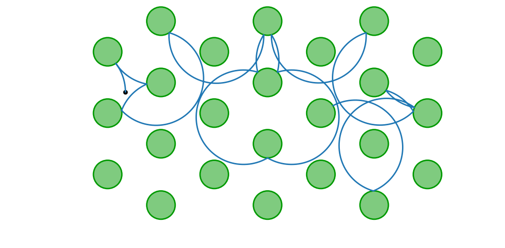
Magnetic and rectangular/hexagonal periodic billiards
using DynamicalBilliards, PyPlot

bd = billiard_hexagonal_sinai(0.4, 1.0; setting = "periodic")

p = MagneticParticle(0.5, 0.6, π/2, 0.75)

xt, yt = timeseries(p, bd, 15)

plot(bd, xt, yt; hexagonal = true)
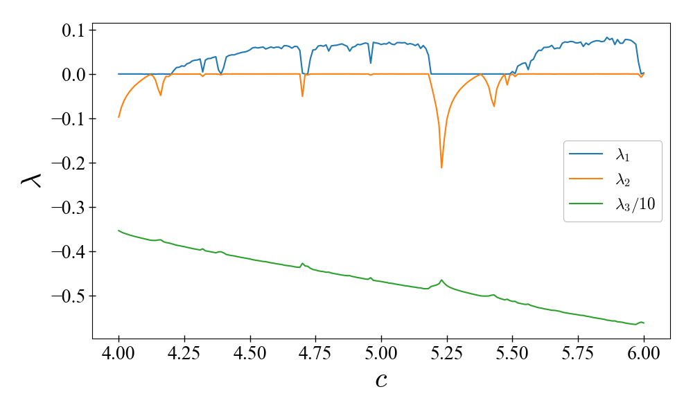
Lyapunov spectrum of the Rössler system
using DynamicalSystems, PyPlot

function roessler(u, p, t)
    a, b, c = p
    du1 = -u[2]-u[3]
    du2 = u[1] + a*u[2]
    du3 = b + u[3]*(u[1] - c)
    return SVector{3}(du1, du2, du3)
end
ds = ContinuousDynamicalSystem(roessler, [0, 1.0, 0], [0.2, 0.2, 5.7])

cs = 4:0.01:6; λs = zeros(length(cs), 3)
for (i, c) in enumerate(cs)
    set_parameter!(ds, 3, c)
    λs[i, :] .= lyapunovs(ds, 10000; Ttr = 500.0)
end

plot(cs, λs)
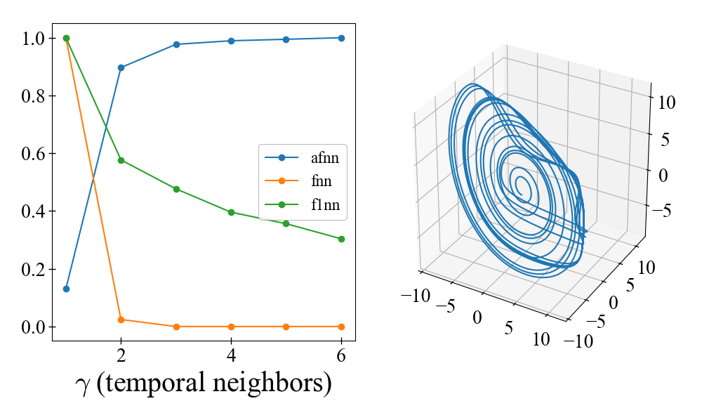
Finding optimal delay time and dimension for the Rössler system
using DynamicalSystems, PyPlot

ds = Systems.roessler()
tr = trajectory(ds, 1000.0; dt = 0.05)

τ = estimate_delay(tr[:, 1], "mi_min") # first minimum of mutual information

figure(figsize = (10, 6)); subplot(1,2,1)
for method in ["afnn", "fnn", "f1nn"]
    Ds = estimate_dimension(tr[:, 1], τ, 1:6, method)
    plot(1:6, Ds ./ maximum(Ds), label = method, marker = "o")
end
legend(); xlabel("\$\\gamma\$ (temporal neighbors)")

subplot(1,2,2, projection = "3d")
rec = embed(tr[:, 1], 4, τ)
plot3D(rec[1:2000, 1],rec[1:2000, 2],rec[1:2000, 3])
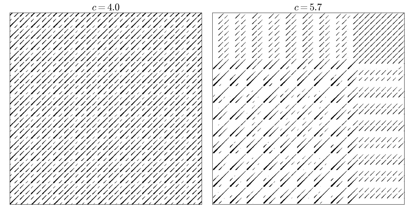
Recurrence matrices of the Rössler system
using DynamicalSystems, PyPlot

ds = Systems.roessler()

for (i, c) in enumerate([4.0, 5.7])
    set_parameter!(ds, 3, c)
    tr = trajectory(ds, 200.0; dt = 0.1, Ttr = 200.0)

    R = RecurrenceMatrix(tr, 3.0)

    subplot(1,2,i)
    imshow(grayscale(R; width = 1000, height = 1000), cmap = "binary_r")
end
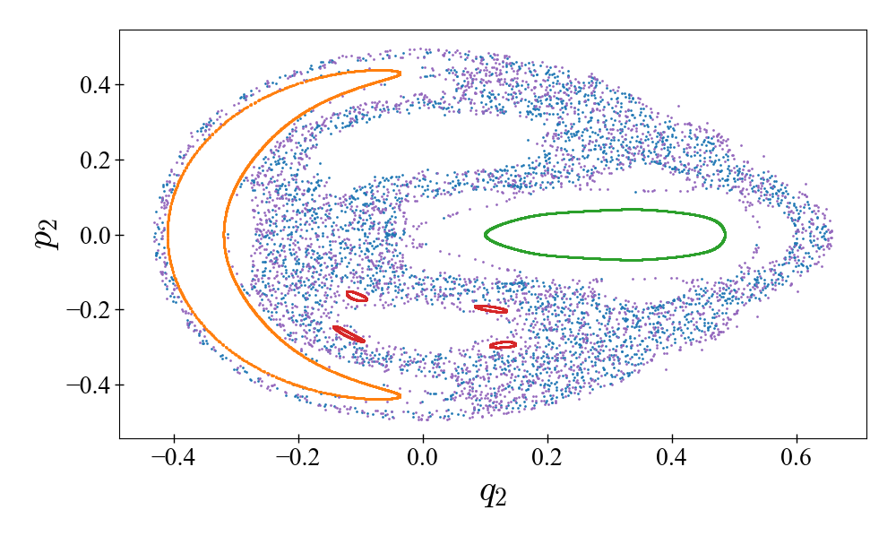
Poincaré surface of section of the Hénon–Heiles system
using DynamicalSystems, PyPlot, OrdinaryDiffEq

hh = Systems.henonheiles()

plane = (1, 0.0)
u0s = [[0.0, -0.25, 0.42081, 0.0],
[0.0, -0.31596, 0.354461, 0.0591255],
[0.0, 0.1, 0.5, 0.0],
[0.0, -0.0910355, 0.459522, -0.173339],
[0.0, -0.205144, 0.449328, -0.0162098]]

for u0 in u0s
    psos = poincaresos(hh, plane, 20000.0; alg = Vern9(), u0 = u0)
    scatter(psos[:, 2], psos[:, 4], s = 2.0)
end
Interactive orbit diagram of the Hénon map
using InteractiveChaos, Makie, DynamicalSystems

i = 1
p_index = 1

ds, p_min, p_max, parname = Systems.henon(), 0.8, 1.4, "a"
t = "orbit diagram for the Hénon map"

interactive_orbitdiagram(ds, p_index, p_min, p_max;
                         parname = parname, title = t)
Agent-based flocking simulation
using Agents, AgentsPlots
pyplot()

model, agent_step!, model_step! = Models.flocking()

function bird_shape(b)
    φ = atan(b.vel[2], b.vel[1])
    xs = [(i ∈ (0, 3) ? 2 : 1) * cos(i * 2π / 3 + φ) for i in 0:3]
    ys = [(i ∈ (0, 3) ? 2 : 1) * sin(i * 2π / 3 + φ) for i in 0:3]
    Shape(xs, ys)
end
bird_color(a) = RGB(0.5, 0, mod1(a.id, 20)/20)

anim = @animate for i in 1:200
    p1 = plotabm(model;
    ac = bird_color, am = bird_shape, as = 10, msw = 0,
    xlims = (0, 100), ylims = (0, 100))
    step!(model, agent_step!, model_step!, 1)
end
mp4(anim, "flocking.mp4", fps = 25)
Getting Started
All packages of JuliaDynamics are registered!
To install them simply press ] to enter the package manager mode and then do:
add PackageName.
To get started with Julia, check out Julia's setup instructions.
For plotting we recommend PyPlot or Makie.