Recurrence Plots
Recurrence Matrices
A Recurrence plot (which refers to the plot of a recurrence matrix) is a way to quantify recurrences that occur in a trajectory. A recurrence happens when a trajectory visits the same neighborhood on the phase space that it was at some previous time.
The central structure used in these recurrences is the (cross-) recurrence matrix:
\[R[i, j] = \begin{cases} 1 \quad \text{if}\quad d(x[i], y[j]) \le \varepsilon\\ 0 \quad \text{else} \end{cases}\]
where $d(x[i], y[j])$ stands for the distance between trajectory $x$ at point $i$ and trajectory $y$ at point $j$. Both $x, y$ can be single timeseries, full trajectories or embedded timeseries (which are also trajectories).
If $x\equiv y$ then $R$ is called recurrence matrix, otherwise it is called cross-recurrence matrix. There is also the joint-recurrence variant, see below. With RecurrenceAnalysis you can use the following functions to access these matrices
RecurrenceAnalysis.RecurrenceMatrix — Type
RecurrenceMatrix(x, rthres; metric = Euclidean(), parallel::Bool)Create a recurrence matrix from timeseries or trajectory x and with recurrence threshold rthres. x is either a StateSpaceSet for multivariate data or an AbstractVector{<:Real} for timeseries.
The variable rthres defines how recurrences are estimated. It can be any subtype of AbstractRecurrenceType, and different types can specify recurrences differently. Alternatively, rthres can be a real number, which then becomes an instance of RecurrenceThreshold.
The keyword metric, if given, must be any subtype of Metric from Distances.jl and defines the metric used to calculate distances for recurrences. By default the Euclidean metric is used, typical alternatives are Chebyshev(), Cityblock().
The keyword parallel decides if the comptutation should be done in parallel using threads. Defaults to length(x) > 500 && Threads.nthreads() > 1.
Description
A (cross-)recurrence matrix is a way to quantify recurrences that occur in a trajectory. A recurrence happens when a trajectory visits the same neighborhood on the state space that it was at some previous time.
The recurrence matrix is a numeric representation of a recurrence plot, described in detail in [Marwan2007] and [Marwan2015]. It represents a a sparse square matrix of Boolean values that quantifies recurrences in the trajectory, i.e., points where the trajectory returns close to itself. Given trajectories x, y, and asumming ε isa Real, the matrix is defined as:
R[i,j] = metric(x[i], y[i]) ≤ ε ? true : falsewith the metric being the distance function. The difference between a RecurrenceMatrix and a CrossRecurrenceMatrix is that in the first case x === y.
Objects of type <:AbstractRecurrenceMatrix are displayed as a recurrenceplot.
See also: CrossRecurrenceMatrix, JointRecurrenceMatrix and use recurrenceplot to turn the result of these functions into a plottable format.
RecurrenceAnalysis.CrossRecurrenceMatrix — Type
CrossRecurrenceMatrix(x, y, rthres; kwargs...)Create a cross recurrence matrix from trajectories x and y. See RecurrenceMatrix for possible value for rthres and kwargs.
The cross recurrence matrix is a bivariate extension of the recurrence matrix. For the time series x, y, of length n and m, respectively, it is a sparse n×m matrix of Boolean values.
Note that cross recurrence matrices are generally not symmetric irrespectively of rthres.
RecurrenceAnalysis.JointRecurrenceMatrix — Type
JointRecurrenceMatrix(x, y, rthres; kwargs...)Create a joint recurrence matrix from trajectories x and y. See RecurrenceMatrix for possible values for rthres and kwargs.
The joint recurrence matrix considers the recurrences of the trajectories of x and y separately, and looks for points where both recur simultaneously. It is calculated by the element-wise multiplication of the recurrence matrices of x and y. If x and y are of different length, the recurrences are only calculated until the length of the shortest one.
See RecurrenceMatrix for details, references and keywords.
JointRecurrenceMatrix(R1::AbstractRecurrenceMatrix, R2::AbstractRecurrenceMatrix)Equivalent with R1 .* R2.
Advanced recurrences specification
RecurrenceAnalysis.AbstractRecurrenceType — Type
AbstractRecurrenceTypeSupertype of all recurrence specification types. Instances of subtypes are given to RecurrenceMatrix and similar constructors to specify recurrences. Use recurrence_threshold to extract the numeric distance threshold.
Possible subtypes are:
RecurrenceThreshold(ε::Real): Recurrences are defined as any point with distance≤ εfrom the referrence point.RecurrenceThresholdScaled(ratio::Real, scale::Function): Herescaleis a function of the distance matrixdm(seedistancematrix) that is used to scale the value of the recurrence thresholdεso thatε = ratio*scale(dm). After the newεis obtained, the method works just like theRecurrenceThreshold. Specialized versions are employed ifscaleismeanormaximum.GlobalRecurrenceRate(q::Real): Here the number of total recurrence rate over the whole matrix is specified to be a quantileq ∈ (0,1)of thedistancematrix. In practice this yields (approximately) a ratioqof recurrences out of the totalNx * Nyfor input trajectoriesx, y.LocalRecurrenceRate(r::Real): The recurrence threhsold here is point-dependent. It is defined so that each point ofxhas a fixed number ofk = r*Nneighbors, with ratiorout of the total possibleN. Equivalently, this means that each column of the recurrence matrix will have exactlyktrue entries. Notice thatLocalRecurrenceRatedoes not guarantee that the resulting recurrence matrix will be symmetric.
RecurrenceAnalysis.RecurrenceThreshold — Type
RecurrenceThreshold(ε::Real)Recurrences are defined as any point with distance ≤ ε from the referrence point. See AbstractRecurrenceType for more.
RecurrenceAnalysis.RecurrenceThresholdScaled — Type
RecurrenceThresholdScaled(ratio::Real, scale::Function)Recurrences are defined as any point with distance ≤ d from the referrence point, where d is a scaled ratio (specified by ratio, scale) of the distance matrix. See AbstractRecurrenceType for more.
RecurrenceAnalysis.GlobalRecurrenceRate — Type
GlobalRecurrenceRate(rate::Real)Recurrences are defined as a constant global recurrence rate. See AbstractRecurrenceType for more.
RecurrenceAnalysis.LocalRecurrenceRate — Type
LocalRecurrenceRate(rate::Real)Recurrences are defined as a constant local recurrence rate. See AbstractRecurrenceType for more.
RecurrenceAnalysis.recurrence_threshold — Function
recurrence_threshold(rt::AbstractRecurrenceType, x [, y] [, metric]) → εReturn the calculated distance threshold ε for rt. The output is real, unless rt isa LocalRecurrenceRate, where ε isa Vector.
Simple Recurrence Plots
The recurrence matrices are internally stored as sparse matrices with Boolean values. Typically in the literature one does not sees the plots of the matrices (hence "Recurrence Plots"). By default, when a Recurrence Matrix is created we "show" a mini plot of it which is a text-based scatterplot.
Here is an example recurrence plot/matrix of a full trajectory of the Roessler system:
using RecurrenceAnalysis, DynamicalSystemsBase

# Create trajectory of Roessler system
@inbounds function roessler_rule(u, p, t)
    a, b, c = p
    du1 = -u[2]-u[3]
    du2 = u[1] + a*u[2]
    du3 = b + u[3]*(u[1] - c)
    return SVector(du1, du2, du3)
end
p0 = [0.15, 0.2, 10.0]
u0 = ones(3)
ro = CoupledODEs(roessler_rule, u0, p0)
N = 2000; Δt = 0.05
X, t = trajectory(ro, N*Δt; Δt, Ttr = 10.0)

# Make a recurrence matrix with fixed threshold
R = RecurrenceMatrix(X, 5.0)
recurrenceplot(R; ascii = true)
(2001, 2001) RecurrenceMatrix with 383575 recurrences of type RecurrenceThreshold.
+------------------------------------------------------------+
| ..:'.::' .::'.:'..:' ..:'.:: .. .:'|
| .. .::'.:'' .:' .:'..''.::' . .::'.:' .:'..:' |
| .:':.:'.::' . .:'.::'.::'.:' .:'.::'.::'.. ::'.::'.:' |
|:'.::'.::' :.:::.:' .. '.::'.::' :.:::.:' |
| ''' ''' ' .. ..:''''' ..:'.. .:''''' ' .. ..:' ''' ..|
| .:'.::' .::'.:'.::' .::'.:'' . .:''|
| .:' .:'..: ..:'..:'.:''.:' .:'..:'..: ..:'.::|
|. ..:'.::'.::' .::'.::' :'.::' .::'.::'.:'' ' .::'.:'' |
|'.::'.::'.:' .:::.:'.. .:'' .:::.:::.:' .:':::' |
|:::::':::' '.::'.:'' ' ':::'.::' '.::'.. |
|'::' ::' .. .::'::' .. . .::'.::' .. .::'::' .|
| .:'.::' .::'.:' .:' ..:'.::' .::'|
| .::'.::'.: .:''.:'.::'.. .::'.:''.: . .:':.:|
| :'' :'.::'.: ::' ::'.:':.:'.. :' ::'.::'.:' ::'.::'.|
| . .:'..:' .:'.::'.:''.:' . ..:'.::' ..:'.::'|
| ..:'.::'.::' .::'.::'..'.::' ..:'.::'.:'' .::'.:'' |
|.::'.:::.:' :::::'.::' :'' :::.:::.:' :':::'.:: |
|::::':::' .::'.::' . .::'.::' .::'.:'' |
| '' '' '.:' .:'' '' .:'..: .:'' ''' .:' .:'' '' .:|
| .:'..:'. .::'.:''.:'.. .:'.::'. . .::'.|
| .::'.::'.:' .:''.:'.::'.:' .::'.:':.:'. .:'..:'|
|. .:':.:'..:' '.::'.::' ''.:' ..:':::'..'' '.::'.::' |
|:::'.::'.:'' :::.::'.. ::' ::'.::'.:' :::.:'' |
|::::::::' .::'.::' .::::::' .::'.:: |
|::::::'.. ::.::' :::::'. ::.:' |
+------------------------------------------------------------+ Or make a recurrence matrix with fixed (global) recurrence rate of 10%
R = RecurrenceMatrix(X, GlobalRecurrenceRate(0.1))
recurrenceplot(R; ascii = true)
(2001, 2001) RecurrenceMatrix with 400401 recurrences of type GlobalRecurrenceRate.
+------------------------------------------------------------+
| ..:'.::' .::'.:'..:' ..:'.:: ... .:'|
| .. .::'.:'' .:' .:'..''.::' .. .::'.:' .:'..:' |
| .:':.:'.::'.. .:'.::'.::'.:' . .:'.::'.::'.. ::'.::'.:' |
|:'.::'.::' :.:::.:' .. '.::'.::' :.:::.:' |
| ''' ''' ' .. ..:''''' ..:'.. .:''''' ' .. ..:' ''' ..|
| .:'.::' .::'.:'.::' .::'.:'' .. .:''|
| .:' .:'..: ..:'..:'.::'.:' .:'..:'.:: ..:'.::|
|. ..:'.::'.::' ' .::'.::' :'.::' .::'.::'.:'' ' .::'.:'' |
|'.::'.::'.:' .:::.:'.. .:'' .:::.:::.:' .:':::' |
|:::::':::' ':::'.:'' ' ':::'.::' '.::'.. |
|'::' ::' .. .::'::' .. .. .::':::' .. .::'::' .|
| .:'.::' .::'.:' .:' ..:'.::' . .::'|
| .::'.::'.: .:''.:'.::'.: .::'.:''.: .. .:':.:|
| :'' :'.::'.:' ::' ::'.:':.:'.. :' ::'.::'.:' ::'.::'.|
| . .:'..:' .:'.::'.:''.:' . ..:'.::' ..:'.::'|
| ..:'.::'.::' .::'.::'..'.::' ..:'.::'.:'' .::'.:'' |
|.:::.:::.:' :::::'.::' ::' :::.:::.:' :':::'.:: |
|::::':::' .::'.::' .. .::'.::' .::'.:'' |
| '' '' '.:: .:'' ''' .:'..: .:'' ''' '.:' .:'' '' .:|
| .:'..:'. .::'.:''.:'.. .:'.::'. : .::'.|
| .::'.::'.:' .:''.:'.::'.:'' .::'.:':.:'. .:'..:'|
|. .:':.:'..:' '.::'.::' ':.:' ..:':::'..:' '.::'.::' |
|:::'.::'.:'' :::.::'.. ::' ::'.::'.:' :::.:'' |
|::::::::' .::'.::' .::::::' .::'.:: |
|::::::'.. ::.::' :::::'. ::.:'' |
+------------------------------------------------------------+ typeof(R)RecurrenceMatrix{GlobalRecurrenceRate{Float64}}summary(R)"(2001, 2001) RecurrenceMatrix with 400401 recurrences of type GlobalRecurrenceRate."The above simple plotting functionality is possible through the package UnicodePlots. The following function creates the plot:
RecurrenceAnalysis.recurrenceplot — Function
recurrenceplot([io,] R; minh = 25, maxh = 0.5, ascii, kwargs...) -> uCreate a text-based scatterplot representation of a recurrence matrix R to be displayed in io (by default stdout) using UnicodePlots. The matrix spans at minimum minh rows and at maximum maxh*displaysize(io)[1] (i.e. by default half the display). As we always try to plot in equal aspect ratio, if the width of the plot is even less, the minimum height is dictated by the width.
The keyword ascii::Bool can ensure that all elements of the plot are ASCII characters (true) or Unicode (false).
The rest of the kwargs are propagated into UnicodePlots.scatterplot.
Notice that the accuracy of this function drops drastically for matrices whose size is significantly bigger than the width and height of the display (assuming each index of the matrix is one character).
Here is the same plot but using Unicode Braille characters
recurrenceplot(R; ascii = false) (2001, 2001) RecurrenceMatrix with 400401 recurrences of type GlobalRecurrenceRate.
┌────────────────────────────────────────────────────────────┐
│⠀⠀⠀⠀⠀⠀⠀⠀⠀⢀⣠⠞⠃⢀⣴⠟⠁⠀⠀⠀⠀⠀⠀⠀⢀⣴⠟⠁⣠⡾⠋⢀⣤⠞⠁⠀⠀⠀⠀⠀⠀⠀⢀⣤⠞⠁⣀⡴⠟⠀⠀⠀⠀⢀⣤⠄⠀⣀⡴⠛│
│⠀⠀⠀⢀⡀⠀⠀⣠⣴⠟⠁⣠⡾⠋⠁⠀⠀⠀⣠⡴⠛⠀⣠⡾⠋⢀⣠⠘⠉⣀⡴⠟⠁⠀⠀⠀⢀⡀⠀⠀⣠⡶⠟⠁⣠⡾⠋⠀⠀⠀⠀⣠⡶⠋⢀⣠⡾⠋⠀⠀│
│⠀⣠⡶⠛⢁⣤⡾⠋⢀⣴⠾⠋⢀⡀⠀⠀⢠⡾⠋⢀⣴⠟⠋⣀⡴⠟⠁⢠⡾⠋⠀⡀⠀⠀⢠⡾⠋⢀⣴⡾⠋⢀⣴⠟⠁⢀⡄⠀⠀⣴⡿⠋⣀⣴⠟⠁⣠⡴⠋⠀│
│⡿⠋⣠⣴⡿⠋⣠⣶⠟⠁⠀⠀⠀⠀⠀⠀⢈⣠⣾⠟⢁⣠⡾⠋⠀⠀⠀⠀⢀⡄⠀⠀⠀⠀⠈⣠⣶⠿⠋⣠⣾⠟⠁⠀⠀⠀⠀⠀⠀⢉⣤⣾⠟⢁⣤⡾⠋⠀⠀⠀│
│⠀⠚⠛⠁⠀⠛⠛⠁⠀⠚⠀⣠⡄⠀⢀⣠⠞⠛⠁⠐⠛⠋⠀⠀⠀⢀⣠⠞⠋⢀⡄⠀⠀⣠⡼⠛⠁⠐⠛⠋⠀⠀⠒⠀⣠⠄⠀⢀⣤⠟⠋⠀⠐⠛⠉⠀⠀⠀⢀⣤│
│⠀⠀⠀⠀⠀⠀⠀⠀⠀⣤⠞⠉⢀⣴⠟⠁⠀⠀⠀⠀⠀⠀⠀⢀⣴⠟⠁⣠⡾⠋⢀⣴⠞⠉⠀⠀⠀⠀⠀⠀⠀⢀⣴⠞⠁⣠⡴⠛⠁⠀⠀⠀⢀⡄⠀⠀⣠⡴⠛⠁│
│⠀⠀⠀⠀⠀⠀⣀⡴⠋⠀⣠⡾⠋⢀⣠⠞⠀⠀⠀⠀⢀⣠⡾⠋⢀⣤⠞⠁⣠⡴⠟⠁⣠⡶⠃⠀⠀⠀⠀⣠⡴⠋⢀⣠⡾⠋⢀⣴⠞⠀⠀⠀⠀⢀⣤⠾⠋⢀⣴⠞│
│⣀⠀⠀⢀⣤⡾⠋⢀⣴⠟⠋⢀⡴⠟⠁⠀⠐⠀⣀⣴⠟⠁⣠⡴⠟⠁⠀⠸⠋⢀⣴⠞⠁⠀⠀⠀⢀⣴⠾⠋⣀⣴⠟⠁⣀⡴⠛⠁⠀⠚⠀⣠⣴⠟⠁⣠⡶⠋⠁⠀│
│⠋⣠⣶⠟⠉⣠⣾⠟⠁⣠⡾⠋⠀⠀⠀⠀⣠⣾⠟⢁⣤⡾⠋⢀⡀⠀⠀⢠⡴⠋⠁⠀⠀⠀⢠⣶⠟⢁⣠⡾⠟⢁⣠⠾⠋⠀⠀⠀⠀⣤⡾⠋⢁⣴⡾⠋⠀⠀⠀⠀│
│⣿⠟⣁⣴⡿⠋⣁⣴⠟⠋⠀⠀⠀⠀⠀⠀⠉⣡⣶⠿⠋⣠⡴⠛⠁⠀⠀⠈⠀⠀⠀⠀⠀⠀⠈⣡⣴⡿⠋⣠⣴⠟⠁⠀⠀⠀⠀⠀⠀⠉⣠⣾⠟⠁⣠⡤⠀⠀⠀⠀│
│⠁⠾⠿⠋⠀⠾⠟⠁⠀⠀⠀⢀⡀⠀⠀⣠⡾⠟⠁⠰⠾⠋⠀⠀⠀⠀⣠⡤⠀⢀⡀⠀⠀⣀⡼⠿⠋⠰⠾⠟⠁⠀⠀⠀⣀⡀⠀⠀⣠⠿⠟⠁⠰⠿⠋⠀⠀⠀⠀⣠│
│⠀⠀⠀⠀⠀⠀⠀⠀⠀⣠⡾⠋⢀⣴⠞⠉⠀⠀⠀⠀⠀⠀⠀⢀⣴⠞⠁⢠⡴⠋⠀⣠⡾⠋⠀⠀⠀⠀⠀⠀⠀⢀⣠⠞⠋⢀⣴⠟⠁⠀⠀⠀⠀⡀⠀⠀⢀⣴⠟⠁│
│⠀⠀⠀⠀⠀⠀⢀⣴⠟⠁⣠⡴⠟⠁⣠⡶⠀⠀⠀⠀⠀⣠⡶⠋⠁⣠⡾⠋⢀⣴⠟⠁⣀⡴⠀⠀⠀⠀⠀⣀⣴⠟⠁⣠⡶⠋⠁⣠⠖⠀⣀⡀⠀⠀⣠⡾⠋⢁⣠⠞│
│⠀⠀⠀⠀⠀⠾⠛⠁⠀⠾⠋⢀⣴⠞⠁⣠⡴⠂⠀⠰⠾⠋⠀⠰⠟⠁⣠⡼⠛⢁⣤⠞⠋⢀⡤⠀⠀⠀⠾⠋⠀⠰⠾⠋⣀⡴⠟⠁⣠⠾⠋⠀⠰⠟⠋⣀⡰⠟⠁⣠│
│⠀⠀⠀⠀⠀⢀⠀⠀⠀⣠⡾⠋⢀⣤⠞⠋⠀⠀⠀⠀⣠⡾⠃⢀⣴⠞⠋⢠⡴⠛⠁⣠⡾⠋⠀⠀⠀⠀⣀⠀⠀⢀⣠⡾⠋⢀⣴⠞⠁⠀⠀⠀⢀⣠⠞⠋⢀⣴⠞⠁│
│⠀⠀⢀⣠⡾⠋⢀⣴⠟⠋⢀⣴⠟⠁⠀⠀⠀⣀⣴⠟⠁⣠⣴⠟⠁⣠⡄⠈⢀⣴⠞⠉⠀⠀⠀⢀⣤⠞⠋⣀⣴⠟⠉⣠⡴⠛⠁⠀⠀⠀⣀⣴⠟⠁⣠⡶⠛⠁⠀⠀│
│⣠⣴⠟⢉⣠⣾⠟⢁⣠⡾⠋⠀⠀⠀⠀⠀⠼⠟⢁⣴⡾⠋⢀⣴⠞⠉⠀⠰⠟⠁⠀⠀⠀⠀⠰⠟⢁⣠⡾⠟⢁⣤⡾⠋⠀⠀⠀⠀⠀⠾⠛⢁⣴⡿⠋⢀⣴⠆⠀⠀│
│⠟⣁⣴⡿⠛⣡⣴⡿⠋⠀⠀⠀⠀⠀⠀⠀⢠⣶⡿⠋⣠⣶⠟⠁⠀⠀⠀⢀⡀⠀⠀⠀⠀⠀⢠⣴⡿⠋⣠⣴⠟⠉⠀⠀⠀⠀⠀⠀⠀⣠⣾⠟⠉⣠⡾⠋⠁⠀⠀⠀│
│⠀⠉⠉⠀⠀⠉⠁⠀⠀⠉⢀⡴⠆⠀⣠⡶⠋⠁⠀⠈⠉⠁⠀⠀⠀⣠⡶⠋⢀⣤⠆⠀⣀⡴⠋⠉⠀⠈⠉⠁⠀⠀⠁⣀⡴⠂⠀⣠⡶⠋⠁⠀⠈⠉⠀⠀⠀⠀⣠⠶│
│⠀⠀⠀⠀⠀⠀⠀⠀⣠⠾⠋⢀⣤⠞⠋⢀⠀⠀⠀⠀⠀⠀⢀⣴⠞⠉⣀⡴⠋⠁⣠⡾⠋⢀⡀⠀⠀⠀⠀⠀⠀⣠⠾⠋⢀⣴⠟⠁⣀⠀⠀⠀⠀⠆⠀⢀⣴⠟⠁⣀│
│⠀⠀⠀⠀⠀⢀⣴⠞⠁⣠⣴⠟⠁⣠⡶⠋⠀⠀⠀⠀⣠⡶⠛⠁⣠⡾⠋⢀⣴⠟⠁⣀⡴⠋⠁⠀⠀⠀⣀⣴⠟⠁⣠⡶⠛⢁⣠⠾⠋⢀⠀⠀⠀⣠⡾⠋⢀⣠⠾⠋│
│⣤⠀⠀⣠⡾⠛⢁⣤⡾⠋⢀⣤⠞⠉⠀⠀⠈⢀⣴⡾⠋⢀⣴⠟⠉⠀⠀⠈⢁⣠⠾⠋⠀⠀⠀⢀⣠⡾⠋⢁⣴⡾⠋⢀⣤⠞⠁⠀⠀⠉⢀⣴⠿⠋⣀⣴⠟⠁⠀⠀│
│⣁⣴⡿⠋⣠⣴⠿⠋⣠⡶⠛⠁⠀⠀⠀⠀⣼⠟⢉⣠⡾⠟⠁⣠⠄⠀⠀⢰⠟⠁⠀⠀⠀⠀⢰⡿⠋⣠⣶⠟⠁⣠⡶⠋⠀⠀⠀⠀⠀⣾⠟⢁⣠⡾⠛⠁⠀⠀⠀⠀│
│⡿⢋⣴⣾⠟⢁⣴⡾⠋⠀⠀⠀⠀⠀⠀⠀⢠⣴⡿⠋⣀⣴⠟⠁⠀⠀⠀⠀⠀⠀⠀⠀⠀⠀⢀⣴⣿⠟⣁⣴⡿⠋⠀⠀⠀⠀⠀⠀⠀⣠⣴⡿⠋⣀⣴⠆⠀⠀⠀⠀│
│⣾⣿⢟⣡⣾⡿⠋⣀⡄⠀⠀⠀⠀⠀⠀⠀⠻⢋⣤⣾⠟⠁⠀⠀⠀⠀⠀⠀⠀⠀⠀⠀⠀⠀⠸⢛⣥⣾⠟⠉⣀⠀⠀⠀⠀⠀⠀⠀⠀⠟⢋⣤⡾⠋⠁⠀⠀⠀⠀⠀│
└────────────────────────────────────────────────────────────┘ As you can see, the Unicode based plotting doesn't display nicely everywhere. It does display perfectly in e.g. VSCode, which is where it is the default printing type.
Advanced Recurrence Plots
A text-based plot is cool, fast and simple. But often one needs the full resolution offered by the data of a recurrence matrix.
There are two more ways to plot a recurrence matrix using RecurrenceAnalysis:
RecurrenceAnalysis.coordinates — Function
coordinates(R) -> xs, ysReturn the coordinates of the recurrence points of R (in indices).
RecurrenceAnalysis.grayscale — Function
grayscale(R [, bwcode]; width::Int, height::Int, exactsize=false)Transform the recurrence matrix R into a full matrix suitable for plotting as a grayscale image. By default it returns a matrix with the same size as R, but switched axes, containing "black" values in the cells that represent recurrent points, and "white" values in the empty cells and interpolating in-between for cases with both recurrent and empty cells, see below.
The numeric codes for black and white are given in a 2-element tuple as a second optional argument. Its default value is (0.0, 1.0), i.e. black is coded as 0.0 (no brightness) and white as 1.0 (full brightness). The type of the elements in the tuple defines the type of the returned matrix. This must be taken into account if, for instance, the image is coded as a matrix of integers corresponding to a grayscale; in such case the black and white codes must be given as numbers of the required integer type.
The keyword arguments width and height can be given to define a custom size of the image. If only one dimension is given, the other is automatically calculated. If both dimensions are given, by default they are adjusted to keep an aspect proportional to the original matrix, such that the returned matrix fits into a matrix of the given dimensions. This automatic adjustment can be disabled by passing the keyword argument exactsize=true.
If the image has different dimensions than R, the cells of R are distributed in a grid with the size of the image, and a gray level between white and black is calculated for each element of the grid, proportional to the number of recurrent points contained in it. The levels of gray are coded as numbers of the same type as the black and white codes.
It is advised to use width, height arguments for large matrices otherwise plots using functions like e.g. heatmap could be misleading.
For example, here is the representation of the above R from the Roessler system using both plotting approaches:
using CairoMakie
fig = Figure(resolution = (1000,500))

ax = Axis(fig[1,1])
xs, ys = coordinates(R)
scatter!(ax, xs, ys; color = :black, markersize = 1)
ax.limits = ((1, size(R, 1)), (1, size(R, 2)));
ax.aspect = 1

ax2 = Axis(fig[1,2]; aspect = 1)
Rg = grayscale(R)
heatmap!(ax2, Rg; colormap = :grays)
fig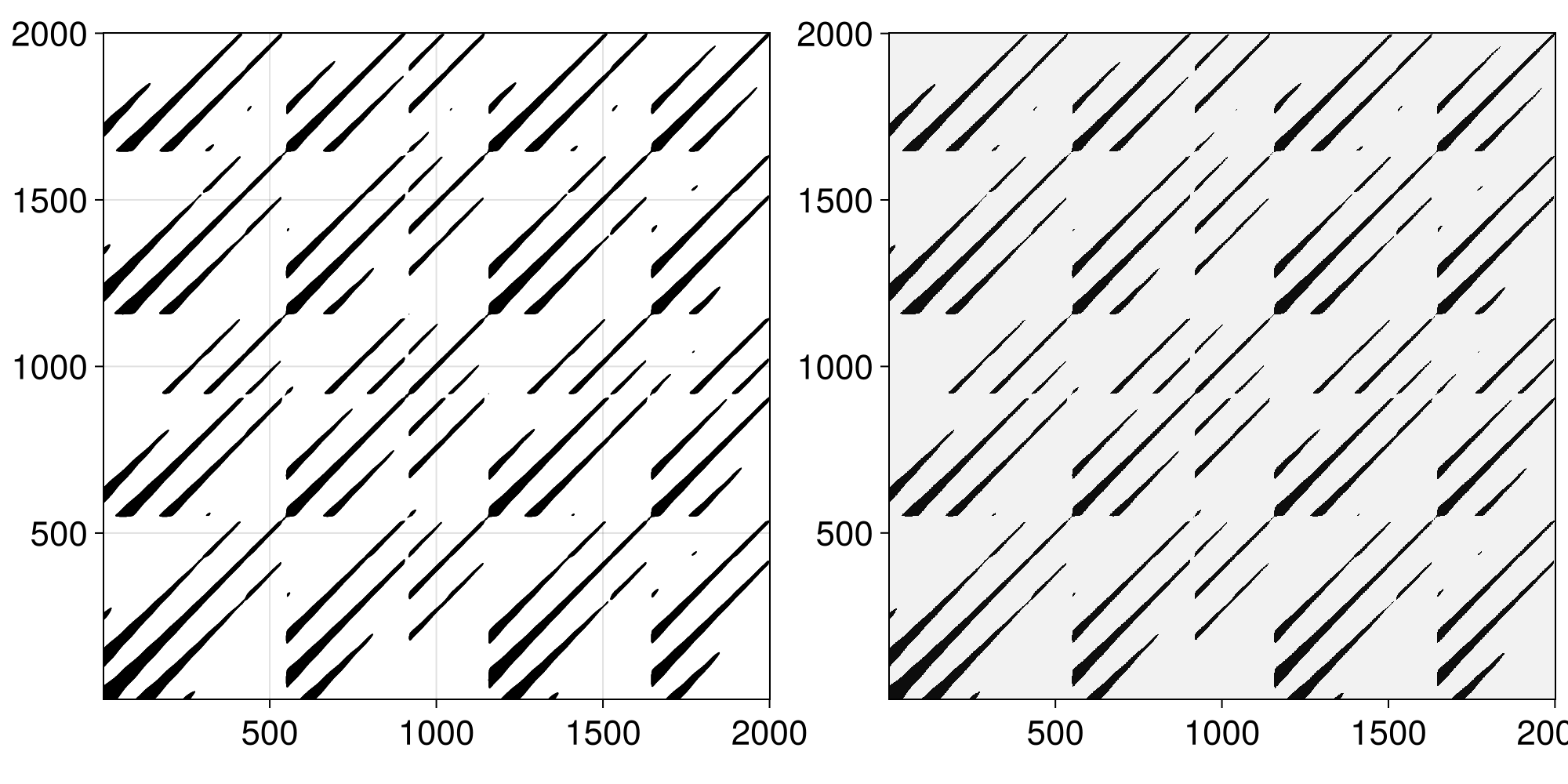
and here is exactly the same process, but using a delay embedded trajectory instead
using DelayEmbeddings

y = X[:, 2]
τ = estimate_delay(y, "mi_min")
m = embed(y, 3, τ)
E = RecurrenceMatrix(m, 5.0; metric = "euclidean")

xs, ys = coordinates(E)
fig, ax = scatter(xs, ys; markersize = 1)
ax.aspect = 1
fig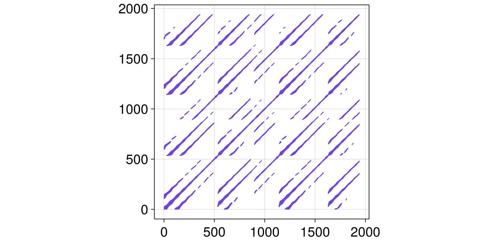
which justifies why recurrence plots are so fitting to be used in embedded timeseries.
It is easy when using grayscale to not change the width/height parameters. The width and height are important when in grayscale when the matrix size exceeds the display size! Most plotting libraries may resample arbitrarily or simply limit the displayed pixels, so one needs to be extra careful.
Besides graphical problems there are also other potential pitfalls dealing with the conceptual understanding and use of recurrence plots. All of these are summarized in the following paper which we suggest users to take a look at:
N. Marwan, How to avoid potential pitfalls in recurrence plot based data analysis, Int. J. of Bifurcations and Chaos (arXiv).
Skeletonized Recurrence Plots
The finite size of a recurrence plot can cause border effects in the recurrence quantification-measures rqa. Also the sampling rate of the data and the chosen recurrence threshold selection method (fixed, fixedrate, FAN) plays a crucial role. They can cause the thickening of diagonal lines in the recurrence matrix. Both problems lead to biased line-based RQA-quantifiers and is discussed in:
K.H. Kraemer & N. Marwan, Border effect corrections for diagonal line based recurrence quantification analysis measures, Phys. Lett. A 2019.
RecurrenceAnalysis.skeletonize — Function
skeletonize(R) → R_skelSkeletonize the RecurrenceMatrix R by using the algorithm proposed by Kraemer & Marwan [Kraemer2019]. This function returns R_skel, a recurrence matrix, which only consists of diagonal lines of "thickness" one.
Consider, e.g. a skeletonized version of a simple sinusoidal:
using RecurrenceAnalysis, DelayEmbeddings, CairoMakie

data = sin.(2*π .* (0:400)./ 60)
Y = embed(data, 3, 15)

R = RecurrenceMatrix(Y, GlobalRecurrenceRate(0.25))
R_skel = skeletonize(R)

fig = Figure(resolution = (1000,600))
ax = Axis(fig[1,1]; title = "RP of monochromatic signal")
heatmap!(ax, grayscale(R); colormap = :grays)

ax = Axis(fig[1,2]; title = "skeletonized RP")
heatmap!(ax, grayscale(R_skel); colormap = :grays)
fig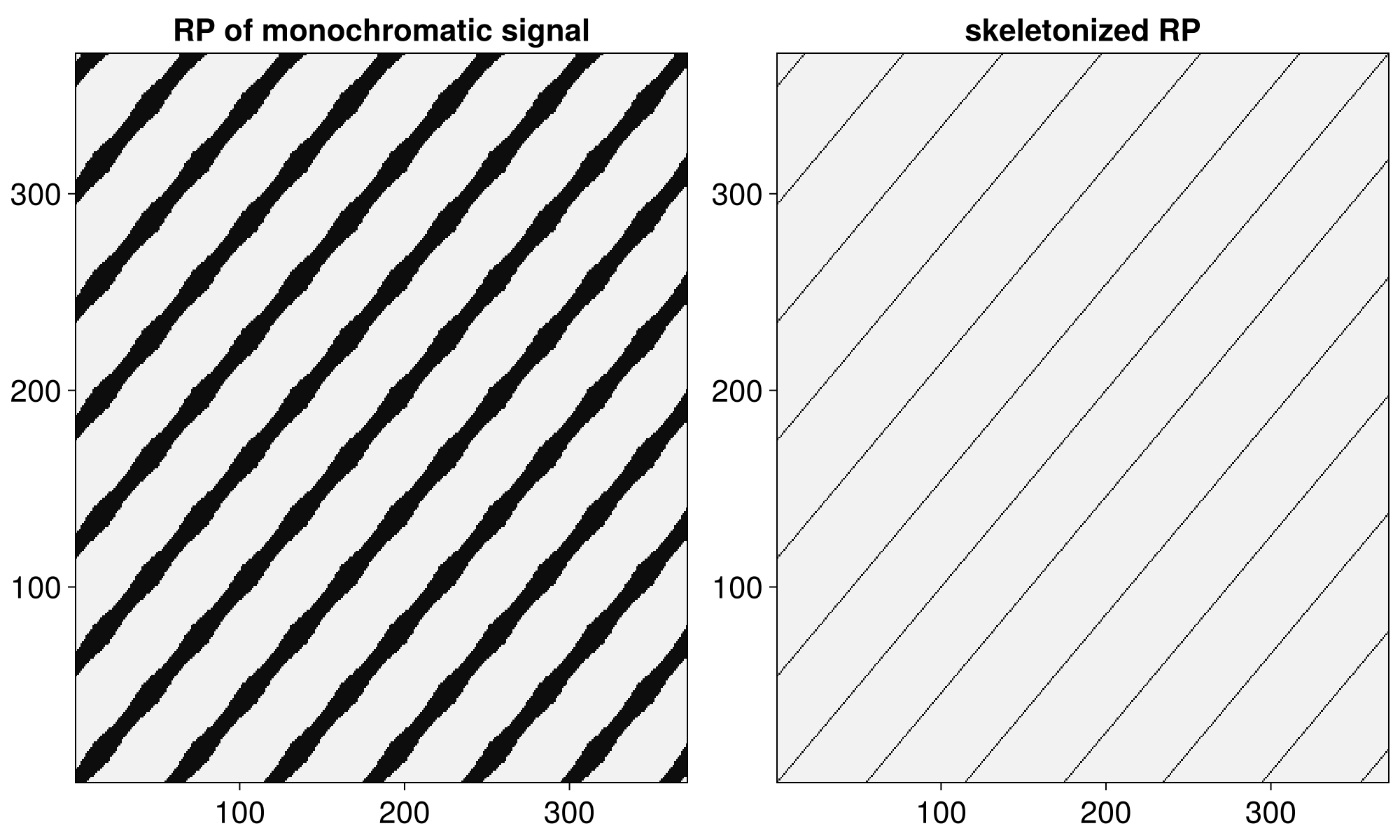
This way spurious diagonal lines get removed from the recurrence matrix, which would otherwise effect the quantification based on these lines.
Distance matrix
The distance function used in RecurrenceMatrix and co. can be specified either as any Metric instance from Distances. In addition, the following function returns a matrix with the cross-distances across all points in one or two trajectories:
RecurrenceAnalysis.distancematrix — Function
distancematrix(x [, y = x], metric = "euclidean")Create a matrix with the distances between each pair of points of the time series x and y using metric.
The time series x and y can be AbstractStateSpaceSets or vectors or matrices with data points in rows. The data point dimensions (or number of columns) must be the same for x and y. The returned value is a n×m matrix, with n being the length (or number of rows) of x, and m the length of y.
The metric can be any of the Metrics defined in the Distances package and defaults to Euclidean().
StateSpaceSet reference
StateSpaceSets.StateSpaceSet — Type
StateSpaceSet{D, T, V} <: AbstractVector{V}A dedicated interface for sets in a state space. It is an ordered container of equally-sized points of length D, with element type T, represented by a vector of type V. Typically V is SVector{D,T} or Vector{T} and the data are always stored internally as Vector{V}. SSSet is an alias for StateSpaceSet.
The underlying Vector{V} can be obtained by vec(ssset), although this is almost never necessary because StateSpaceSet subtypes AbstractVector and extends its interface. StateSpaceSet also supports almost all sensible vector operations like append!, push!, hcat, eachrow, among others. When iterated over, it iterates over its contained points.
Construction
Constructing a StateSpaceSet is done in three ways:
- By giving in each individual columns of the state space set as
Vector{<:Real}:StateSpaceSet(x, y, z, ...). - By giving in a matrix whose rows are the state space points:
StateSpaceSet(m). - By giving in directly a vector of vectors (state space points):
StateSpaceSet(v_of_v).
All constructors allow for two keywords:
containerwhich sets the type ofV(the type of inner vectors). At the moment options are onlySVector,MVector, orVector, and by defaultSVectoris used.nameswhich can be an iterable of lengthDwhose elements areSymbols. This allows assigning a name to each dimension and accessing the dimension by name, see below.namesisnothingif not given. UseStateSpaceSet(s; names)to add names to an existing sets.
Description of indexing
When indexed with 1 index, StateSpaceSet behaves exactly like its encapsulated vector. i.e., a vector of vectors (state space points). When indexed with 2 indices it behaves like a matrix where each row is a point.
In the following let i, j be integers, typeof(X) <: AbstractStateSpaceSet and v1, v2 be <: AbstractVector{Int} (v1, v2 could also be ranges, and for performance benefits make v2 an SVector{Int}).
X[i] == X[i, :]gives theith point (returns anSVector)X[v1] == X[v1, :], returns aStateSpaceSetwith the points in those indices.X[:, j]gives thejth variable timeseries (or collection), asVectorX[v1, v2], X[:, v2]returns aStateSpaceSetwith the appropriate entries (first indices being "time"/point index, while second being variables)X[i, j]value of thejth variable, at theith timepoint
In all examples above, j can also be a Symbol, provided that names has been given when creating the state space set. This allows accessing a dimension by name. This is provided as a convenience and it is not an optimized operation, hence recommended to be used primarily with X[:, j::Symbol].
Use Matrix(ssset) or StateSpaceSet(matrix) to convert. It is assumed that each column of the matrix is one variable. If you have various timeseries vectors x, y, z, ... pass them like StateSpaceSet(x, y, z, ...). You can use columns(dataset) to obtain the reverse, i.e. all columns of the dataset in a tuple.
- Marwan2007N. Marwan et al., "Recurrence plots for the analysis of complex systems", Phys. Reports 438*(5-6), 237-329 (2007)
- Marwan2015N. Marwan & C.L. Webber, Recurrence Quantification Analysis. Theory and Best Practices Springer (2015)
- Kraemer2019Kraemer, K.H., Marwan, N. (2019). Border effect corrections for diagonal line based recurrence quantification analysis measures. Physics Letters A 383(34).