Distributions

This section introduces the computation of Recurrence Microstates Analysis (RMA) distributions using RecurrenceMicrostatesAnalysis.jl.

We begin with a Quick start with RecurrenceMicrostatesAnalysis.jl, which demonstrates a simple application example. Next, we present A brief review of Recurrence Plots (RP) and RMA. Finally, we explain the distribution function in Computing RMA distributions, including the role of Histograms.

Quick start with RecurrenceMicrostatesAnalysis.jl

This section presents concise examples illustrating how to use the package. RMA distributions are computed using the distribution function, which returns a Probabilities structure containing the microstate distribution.

We start with a simple example based on a uniform random process. First, we generate the data and convert it into a StateSpaceSet:

using Distributions, RecurrenceMicrostatesAnalysis
data = rand(Uniform(0, 1), 10_000);
ssset = StateSpaceSet(data)

1-dimensional StateSpaceSet{Float64} with 10000 points
 0.28769478368805634
 0.3270312001740592
 0.8762853878338924
 0.022373842486420492
 0.6444688570573011
 0.3995735932242024
 0.43763516491971943
 0.24545837329781994
 0.1739045528719606
 0.8475601713614623
 ⋮
 0.15006206550700574
 0.35127293917374447
 0.823147175449717
 0.9025771188676037
 0.6613568435448977
 0.41021813200489277
 0.981946572913893
 0.18291558665176633
 0.6353629851762662

Next, we compute the RMA distribution. This requires specifying the recurrence threshold $\varepsilon$ and the microstate size $N$. These parameters are discussed in more detail in A brief review and Optimizing a parameter.

ε = 0.27
N = 2
dist = distribution(ssset, ε, N)

 Probabilities{Float64,1} over 16 outcomes
  1  0.11082574298344809
  2  0.047184227408636245
  3  0.04726184291621466
  4  0.08552848859202068
  5  0.04713421741663985
  6  0.08556669622590593
  7  0.07679594382957715
  8  0.030660525973089423
  9  0.047239838519736246
 10  0.0769313708879034
 11  0.08582194722505557
 12  0.030578109506279354
 13  0.08565031293252391
 14  0.030441482208145187
 15  0.030611316140964965
 16  0.08176793723385932

As another example, we use DynamicalSystems.jl to generate data from the Hénon map, following the example presented in its documentation:

using DynamicalSystems

function henon_rule(u, p, n) # here `n` is "time", but we don't use it.
    x, y = u # system state
    a, b = p # system parameters
    xn = 1.0 - a*x^2 + y
    yn = b*x
    return SVector(xn, yn)
end

u0 = [0.2, 0.3]
p0 = [1.4, 0.3]

henon = DeterministicIteratedMap(henon_rule, u0, p0)

total_time = 10_000
X, t = trajectory(henon, total_time)
X

2-dimensional StateSpaceSet{Float64} with 10001 points
  0.2        0.3
  1.244      0.06
 -1.10655    0.3732
 -0.341035  -0.331965
  0.505208  -0.102311
  0.540361   0.151562
  0.742777   0.162108
  0.389703   0.222833
  1.01022    0.116911
 -0.311842   0.303065
  ⋮         
 -0.582534   0.328346
  0.853262  -0.17476
 -0.194038   0.255978
  1.20327   -0.0582113
 -1.08521    0.36098
 -0.287758  -0.325562
  0.558512  -0.0863275
  0.476963   0.167554
  0.849062   0.143089

Finally, we compute the RMA distribution of the trajectory X. Here, the threshold is selected using optimize by maximizing the recurrence microstate entropy:

ε, S = optimize(Threshold(), RecurrenceEntropy(), X, N)

(0.8568661000572908, 2.608204784592693)

dist = distribution(X, ε, N)

 Probabilities{Float64,1} over 16 outcomes
  1  0.0512218
  2  0.0278322
  3  0.0548976
  4  0.0533404
  5  0.0547514
  6  0.0531694
  7  0.106138
  8  0.0415038
  9  0.0155716
 10  0.132076
 11  0.0652664
 12  0.0420656
 13  0.0652942
 14  0.0418562
 15  0.0288536
 16  0.1661618

A brief review

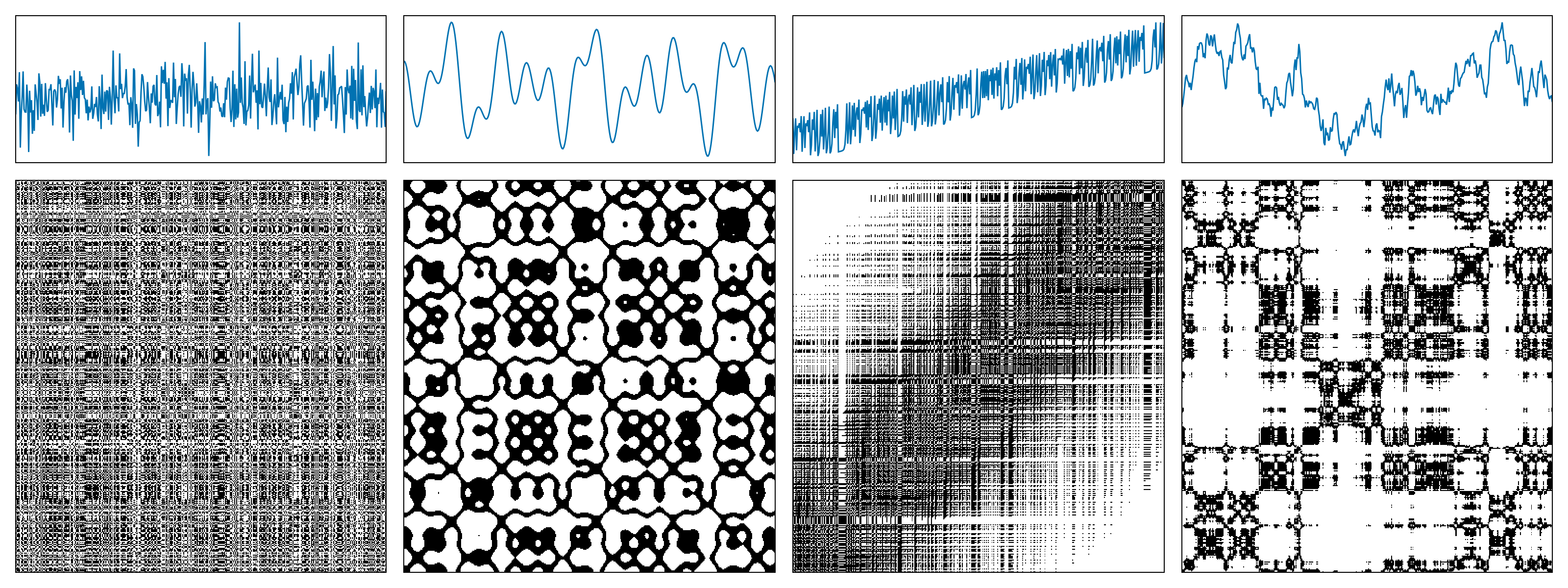
Recurrence Plots (RPs) were introduced in 1987 by Eckmann et al. (Eckmann et al., 1987) as a method for analyzing dynamical systems through recurrence properties.

Consider a time series $\vec{x}_i \in \mathbb{R}^d$, $i \in \{1, 2, \dots, K\}$, where $K$ is the length of the time series and $d$ is the dimension of the phase space. The recurrence plot is defined by the recurrence matrix

\[R_{i,j} = \Theta(\varepsilon - \|\vec x_i - \vec x_j\|),\]

where $\Theta(\cdot)$ denotes the Heaviside step function and $\varepsilon$ is the recurrence threshold.

The following figure shows examples of recurrence plots for different systems: (a) white noise; (b) a superposition of harmonic oscillators; (c) a logistic map with a linear trend; (d) Brownian motion.

A recurrence microstate is a local structure extracted from an RP. For a given microstate shape and size, the set of possible microstates is finite. For example, square microstates with size $N = 2$ yield $16$ distinct configurations.

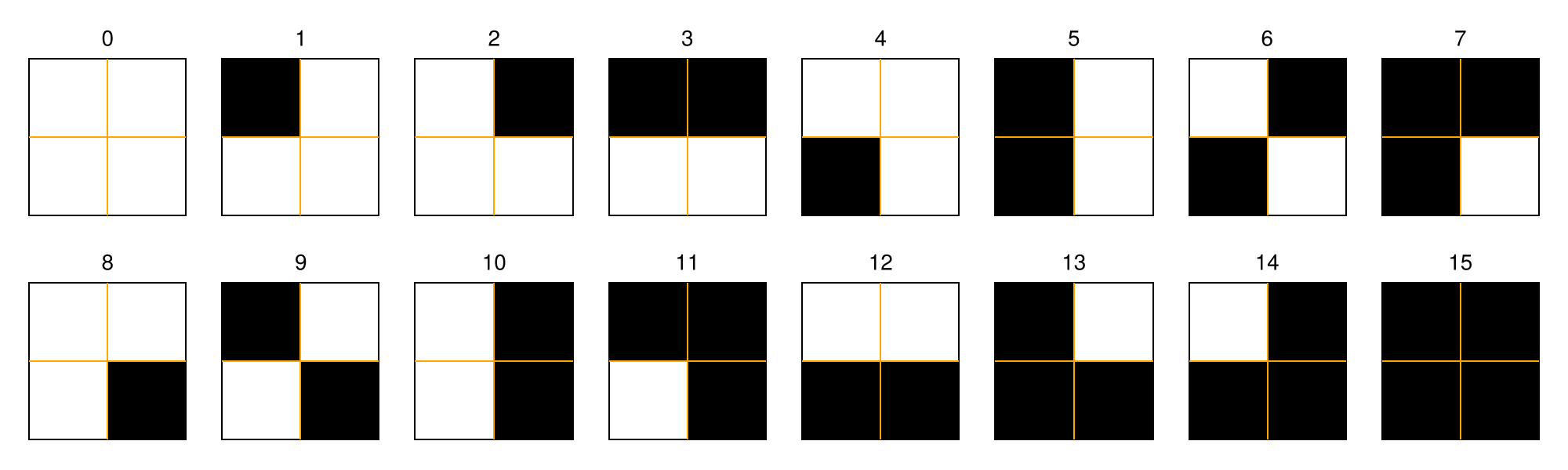
Recurrence Microstates Analysis (RMA) uses the probability distribution of these microstates as a source of information for characterizing dynamical systems.

Computing RMA distributions

The computation of RMA distributions is the core functionality of RecurrenceMicrostatesAnalysis.jl. All other tools in the package rely on these distributions as their primary source of information.

RMA distributions are computed using the distribution function:

distribution(core::RMACore, [x], [y])

distribution(core::CPUCore, [x], [y]; kwargs...)

ssset = StateSpaceSet(rand(Float64, (1000)))
core = CPUCore(Rect(Standard(0.27), 2), SRandom(0.05))
dist = distribution(core, ssset, ssset)

spatialdata = rand(Float64, (3, 50, 50))
core = CPUCore(Rect(Standard(0.5), (2, 2, 1, 1)), SRandom(0.05))
dist = distribution(core, spatialdata, spatialdata)

distribution(core::GPUCore, [x], [y]; kwargs...)

using CUDA
gpudata = StateSpaceSet(Float32.(data)) |> CuVector
core = GPUCore(CUDABackend(), Rect(Standard(0.27f0; metric = GPUEuclidean()), 2), SRandom(0.05))
dist = distribution(core, gpudata, gpudata)

A commonly used convenience interface is:

distribution([x], ε::Float, n::Int; kwargs...)

This method automatically selects a CPUCore when x is a StateSpaceSet and a GPUCore when x is an AbstractGPUVector. By default, square microstates of size n are used.

Additional keyword arguments include:

• rate::Float64: Sampling rate (default: 0.05).
• sampling::SamplingMode: Sampling mode (default: SRandom).
• metric::Metric: Distance metric from Distances.jl. When using a GPUCore, a GPUMetric must be provided.

Alternatively, a RecurrenceExpression can be specified directly:

distribution([x], expr::RecurrenceExpression, n::Int; kwargs...)

Example:

expr = Corridor(0.05, 0.27)
dist = distribution(ssset, expr, 2)

 Probabilities{Float64,1} over 16 outcomes
  1  0.17799396319384614
  2  0.08094677316527843
  3  0.08095877556335757
  4  0.06394477616627803
  5  0.08103439067125612
  6  0.06382355194567875
  7  0.056042997390878695
  8  0.024357466621831043
  9  0.08099738327717879
 10  0.05581755234695892
 11  0.06389956713351327
 12  0.0242482447993109
 13  0.06402619243324817
 14  0.024460087125407655
 15  0.024206236406033924
 16  0.033242041759943636

If a custom MicrostateShape is required, the call simplifies to:

distribution([x], shape::MicrostateShape; kwargs...)

Example:

shape = Triangle(Standard(0.27), 3)
dist = distribution(ssset, shape)

 Probabilities{Float64,1} over 64 outcomes
  1  0.03494116947955793
  2  0.027660258571376835
  3  0.013955379360668395
  4  0.013126047793908004
  5  0.015479788819570064
  6  0.011611242174621414
  7  0.02598578911848957
  8  0.0235634206555781
  9  0.013023406758021857
 10  0.01157522777606487
  ⋮  
 56  0.006926169082399143
 57  0.02146878321953117
 58  0.02094277292061366
 59  0.007587233375903686
 60  0.008456380861068254
 61  0.008105240475141962
 62  0.007927169282279056
 63  0.02031052014595435
 64  0.021231288269049967

Cross-recurrence plots

RMA distributions can also be computed from Cross-Recurrence Plots (CRPs) by providing two time series:

distribution([x], [y], expr::RecurrenceExpression, n::Int; kwargs...)
distribution([x], [y], shape::MicrostateShape; kwargs...)

Example:

data_1 = StateSpaceSet(rand(Uniform(0, 1), 1000))
data_2 = StateSpaceSet(rand(Uniform(0, 1), 2000))
dist = distribution(data_1, data_2, 0.27, 2)

 Probabilities{Float64,1} over 16 outcomes
  1  0.11120569648776678
  2  0.04891288019148531
  3  0.04990435749266407
  4  0.0823326756867733
  5  0.048972969724890084
  6  0.08534716727924607
  7  0.07302881293126759
  8  0.03192757208240278
  9  0.0499844768705371
 10  0.07262821604190244
 11  0.08591801784659142
 12  0.03148691550410111
 13  0.0827533024206067
 14  0.031206497681545504
 15  0.030926079858989895
 16  0.08346436189922986

data_1 = StateSpaceSet(rand(Uniform(0, 1), (1000, 2)))
data_2 = StateSpaceSet(rand(Uniform(0, 1), (2000, 3)))
dist = distribution(data_1, data_2, 0.27, 2)

Spatial data

The package also provides experimental support for spatial data, following "Generalised Recurrence Plot Analysis for Spatial Data" (Marwan et al., 2007). In this context, input data are provided as AbstractArrays:

\[ \vec{x}_{\vec i} \in \mathbb{R}^m,\quad \vec{i} \in \mathbb{Z}^d\]

For example:

spatialdata = rand(Uniform(0, 1), (2, 50, 50))

2×50×50 Array{Float64, 3}:
[:, :, 1] =
 0.0108399  0.132402  0.0573931  0.813676   …  0.905534  0.144873  0.233635
 0.989935   0.712167  0.0762763  0.0811511     0.313637  0.730853  0.463623

[:, :, 2] =
 0.421137  0.00382678  0.229889  0.405717  …  0.970142  0.501561  0.290975
 0.339744  0.971731    0.203877  0.107703     0.846328  0.207389  0.997047

[:, :, 3] =
 0.28056  0.501925  0.995227  0.108032   …  0.637218  0.470099  0.151813
 0.1607   0.420132  0.924564  0.0215797     0.247394  0.555203  0.421879

;;; … 

[:, :, 48] =
 0.705112  0.8773   0.753606   0.211476  …  0.506887  0.759426  0.964074
 0.586371  0.98676  0.0166541  0.490767     0.166902  0.266415  0.0865137

[:, :, 49] =
 0.154691  0.860645  0.901434  0.606442    …  0.930763  0.780562  0.84894
 0.528297  0.373878  0.666882  0.00620051     0.997089  0.710053  0.0468884

[:, :, 50] =
 0.629583  0.106897  0.415768   0.156681  …  0.353183  0.883065  0.804375
 0.309527  0.276529  0.0549814  0.702925     0.555765  0.665665  0.97128

Due to the high dimensionality of spatial recurrence plots, direct visualization is often infeasible. RMA distributions provide a compact alternative by sampling microstates directly from the data.

Examples:

• Full $2 \times d$ microstates:

distribution(spatialdata, Rect(Standard(0.27), (2, 2, 2, 2)))

 Probabilities{Float64,1} over 65536 outcomes
     1  0.0524803896739187
     2  0.008791254540471341
     3  0.008923088665387645
     4  0.0023695449294167032
     5  0.008871048879236473
     6  0.0022030176137329527
     7  0.0022966892288050623
     8  0.0008048820258047953
     9  0.008961251175231838
    10  0.002397299482030662
     ⋮  
 65528  0.0
 65529  0.0
 65530  0.0
 65531  0.0
 65532  0.0
 65533  0.0
 65534  0.0
 65535  0.0
 65536  0.0

spatialdata_1 = rand(Uniform(0, 1), (2, 50, 50))
spatialdata_2 = rand(Uniform(0, 1), (2, 25, 25))
distribution(spatialdata_1, spatialdata_2, Rect(Standard(0.27), (2, 2, 2, 2)))

 Probabilities{Float64,1} over 65536 outcomes
     1  0.05005133841414915
     2  0.00827199236431474
     3  0.007867069661166466
     4  0.002255997917540384
     5  0.007606762209142576
     6  0.0024584592691145207
     7  0.0027766128215881646
     8  0.0008966145569711782
     9  0.008055069487628165
    10  0.0023283055431025756
     ⋮  
 65528  0.0
 65529  0.0
 65530  0.0
 65531  0.0
 65532  0.0
 65533  0.0
 65534  0.0
 65535  0.0
 65536  0.0

• Projected microstates:

distribution(spatialdata, Rect(Standard(0.27), (2, 1, 2, 1)))

 Probabilities{Float64,1} over 16 outcomes
  1  0.4642065805914202
  2  0.0951070387338609
  3  0.09467388588088296
  4  0.02374344023323615
  5  0.09461391087047064
  6  0.024139941690962098
  7  0.021947521865889212
  8  0.002838817159516868
  9  0.09579341940857976
 10  0.022337359433569345
 11  0.024203248646397335
 12  0.002982090795501874
 13  0.023880049979175342
 14  0.0028554768846314037
 15  0.0029687630154102457
 16  0.0037084548104956267

distribution(spatialdata_1, spatialdata_2, Rect(Standard(0.27), (2, 1, 2, 1)))

 Probabilities{Float64,1} over 16 outcomes
  1  0.4470340136054422
  2  0.09722448979591837
  3  0.09484353741496598
  4  0.02383673469387755
  5  0.09995918367346938
  6  0.02634013605442177
  7  0.02414965986394558
  8  0.0031156462585034015
  9  0.0987891156462585
 10  0.02346938775510204
 11  0.025904761904761906
 12  0.0031020408163265306
 13  0.022965986394557825
 14  0.0030068027210884353
 15  0.002993197278911565
 16  0.0032653061224489797

Histograms

The histogram function counts the occurrences of each microstate identified during sampling. It is called internally by distribution , which converts the resulting Counts into Probabilities.

histogram(core::RMACore, [x], [y])

histogram(core::StandardCPUCore, [x], [y]; kwargs...)

ssset = StateSpaceSet(rand(Float64, (1000)))
core = CPUCore(Rect(Standard(0.27), 2), SRandom(0.05))
dist = histogram(core, ssset, ssset)

spatialdata = rand(Float64, (3, 50, 50))
core = CPUCore(Rect(Standard(0.5), (2, 2, 1, 1)), SRandom(0.05))
dist = histogram(core, spatialdata, spatialdata)

histogram(core::StandardGPUCore, [x], [y]; kwargs...)

using CUDA
gpudata = StateSpaceSet(Float32.(data)) |> CuVector
core = GPUCore(CUDABackend(), Rect(Standard(0.27f0; metric = GPUEuclidean()), 2), SRandom(0.05))
dist = histogram(core, gpudata, gpudata)