Quantifiers
Quantifiers are measures used to characterize specific properties of a dynamical system. Currently, Recurrence Microstates Analysis (RMA) provides five quantifiers that can be computed or estimated from a microstate distribution.
Three of these correspond to classical Recurrence Quantification Analysis (RQA) measures: recurrence rate, determinism, and laminarity. One is an information-theoretic entropy measure. The final quantifier is disorder, which is defined directly in terms of the microstate distribution and exploits symmetry properties of recurrence structures.
All quantifiers implemented in the package inherit from QuantificationMeasure, and their computation is performed using the measure function.
RecurrenceMicrostatesAnalysis.QuantificationMeasure — Type
QuantificationMeasureAbstract supertype defining an RQA or RMA quantification measure.
All quantifiers implemented in the package subtype QuantificationMeasure and define their computation via the measure function.
Implementations
RecurrenceMicrostatesAnalysis.measure — Function
measure(qm::QuantificationMeasure, [...])Compute the quantification measure defined by the given QuantificationMeasure instance.
The accepted arguments ([...]) depend on the specific quantifier implementation.
Recurrence microstates entropy
The Recurrence Microstates Entropy (RME) was introduced in 2018 and marks the starting point of the RMA framework (Corso et al., 2018). It is defined as the Shannon entropy of the RMA distribution:
\[RME = -\sum_{i = 1}^{2^\sigma} p_i^{(N)} \ln p_i^{(N)},\]
where $n$ is the microstate size, $\sigma$ is the number of recurrence elements constrained within the microstate (e.g. $\sigma = n^2$ for square microstates), and $p_i^{(N)}$ denotes the probability of the microstate with decimal representation $i$.
In RecurrenceMicrostatesAnalysis.jl, the RME is implemented by the RecurrenceEntropy struct.
RecurrenceMicrostatesAnalysis.RecurrenceEntropy — Type
RecurrenceEntropy <: QuantificationMeasureDefine the Recurrence Microstates Entropy (RME) quantification measure (Corso et al., 2018).
RME can be computed either from a distribution of recurrence microstates or directly from time-series data. In both cases, the computation is performed via the measure function.
Using a distribution
measure(::RecurrenceEntropy, dist::Probabilities)Arguments
dist: A distribution of recurrence microstates.
Returns
A Float64 corresponding to the RME computed using the Shannon entropy.
Examples
using RecurrenceMicrostatesAnalysis, Distributions
data = StateSpaceSet(rand(Uniform(0, 1), 1000))
dist = distribution(data, 0.27, 3)
rme = measure(RecurrenceEntropy(), dist)
Using a time series
measure(::RecurrenceEntropy, [x]; kwargs...)Arguments
[x]: Time-series data provided as anStateSpaceSet.
Returns
A Float64 corresponding to the maximum RME computed using the Shannon entropy.
Keyword Arguments
N: Integer defining the microstate size. The default value is3.
Examples
using RecurrenceMicrostatesAnalysis, Distributions
data = StateSpaceSet(rand(Uniform(0, 1), 1000))
rme = measure(RecurrenceEntropy(), data; N = 4)Since the output of the distribution function is a Probabilities object, the package also supports other information or complexity measures provided by ComplexityMeasures.jl.
Quick example
As an example, consider a uniform random process. The RME as a function of the threshold can be computed and visualized as follows:
using RecurrenceMicrostatesAnalysis, Distributions, CairoMakie

data_len = 10000
resolution = 50

data = StateSpaceSet(rand(Uniform(0, 1), data_len))
thres_range = range(0, 1, resolution)
results = zeros(Float64, resolution)

for i ∈ eachindex(results)
    dist = distribution(data, thres_range[i], 4)
    results[i] = measure(RecurrenceEntropy(), dist)
end

results ./= maximum(results)
scatterlines(thres_range, results)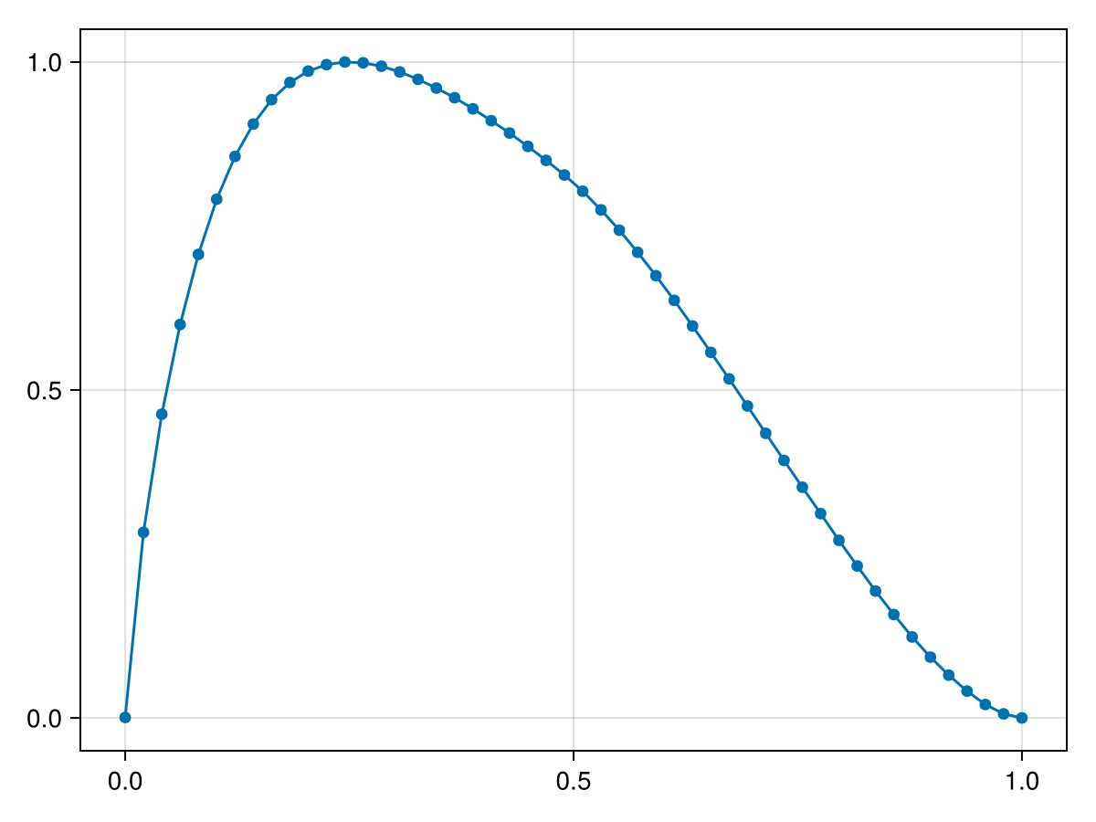
Recurrence rate
The Recurrence Rate (RR) quantifies the density of recurrence points in a recurrence plot (Webber and Marwan, 2015). In standard RQA, it is defined as
\[RR = \frac{1}{K^2} \sum_{i,j=1}^K R_{i,j}.\]
where $K$ is the length of the time series.
When estimated using RMA, RR is defined as the expected recurrence rate over the microstate distribution:
\[RR = \sum_{i = 1}^{2^\sigma} p_i^{(N)} RR_i^{(N)},\]
where $RR_i^{(N)}$ denotes the recurrence rate of the $i$-th microstate. For square microstates, this quantity is given by
\[RR_i^{(N)} = \frac{1}{\sigma} \sum_{j,k=1}^N M_{j,k}^{i, (N)},\]
with $\mathbf{M}^{i, (N)}$ denoting the microstate structure corresponding to index $i$.
In RecurrenceMicrostatesAnalysis.jl, RR is implemented by RecurrenceRate struct.
RecurrenceMicrostatesAnalysis.RecurrenceRate — Type
RecurrenceRate <: QuantificationMeasureDefine the Recurrence Rate (RR) quantification measure.
RR can be computed either from a distribution of recurrence microstates or directly from time-series data. In both cases, the computation is performed via the measure function.
Using a distribution
measure(::RecurrenceRate, dist::Probabilities)Arguments
dist: A distribution of recurrence microstates.
Returns
A Float64 corresponding to the estimated recurrence rate.
Examples
using RecurrenceMicrostatesAnalysis, Distributions
data = StateSpaceSet(rand(Uniform(0, 1), 1000))
dist = distribution(data, 0.27, 3)
rr = measure(RecurrenceRate(), dist)
Using a time series
measure(::RecurrenceRate, [x]; kwargs...)Arguments
[x]: Time-series data provided as aStateSpaceSet.
Returns
A Float64 corresponding to the estimated recurrence rate.
Keyword Arguments
N: Integer defining the microstate size. The default value is3.threshold: Threshold used to compute the RMA distribution. By default, this is chosen as the threshold that maximizes the recurrence microstate entropy (RME).
Examples
using RecurrenceMicrostatesAnalysis, Distributions
data = StateSpaceSet(rand(Uniform(0, 1), 1000))
rme = measure(RecurrenceRate(), data; N = 4)Determinism
In standard RQA, Determinism (DET) measures the fraction of recurrence points forming diagonal line structures (Webber and Marwan, 2015):
\[DET = \frac{\sum_{l=d_{min}}^K l~H_D(l)}{\sum_{i,j=1}^K R_{i,j}},\]
where $H_D(l)$ is the histogram of diagonal line lengths,
\[H_D(l)=\sum_{i,j]1}^K(1-R_{i-1,j-1})(1-R_{i+l,j+l})\prod_{k=0}^{l-1}R_{i+k,j+k}.\]
The estimation of DET using RMA is based on the work "Density-Based Recurrence Measures from Microstates" (da Cruz et al., 2025). In that work, the DET expression is rewritten as
\[DET = 1 - \frac{1}{K^2~RR}\sum_{l=1}^{l_{min}-1} l~H_D(l),\]
and the diagonal histogram $H_D(l)$ is related to the RMA distribution through correlations between microstate structures:
\[\frac{H_D(l)}{(K-l-1)^2}=\vec d^{(l)}\cdot\mathcal{R}^{(l+2)}\vec p^{(l+2)}.\]
For the commonly used case $l_{min} = 2$ (currently the only case implemented in the package), this leads to the approximation
\[DET\approx 1 - \frac{\vec d^{(1)}\cdot\mathcal{R}^{(3)}\vec p^{3}}{RR}.\]
The correlation term $\vec d^{(1)}\cdot\mathcal{R}^{(3)}\vec p^{3}$ can be simplified by explicitly identifying the microstates selected by $\vec d^{(1)}$. These correspond to microstates of the form
\[\begin{pmatrix} \xi & \xi & 0 \\ \xi & 1 & \xi \\ 0 & \xi & \xi \\ \end{pmatrix},\]
where $\xi$ denotes an unconstrained entry. There are $64$ such microstates among the $512$ possible square microstates of size $N = 3$. Defining the class $C_D$ as the set of microstates with this structure, DET can be estimated as:
\[DET\approx 1 - \frac{\sum_{i\in C_D} p_i^{(3)}}{RR},\]
where $p_i^{(3)}$ is the probability of the $i$-th microstate in an RMA distribution of square microstates with size $N = 3$.
A futher simplification can be obtained by defining Diagonal-shaped microstates (Ferreira et al., 2025). In the structure above, the unconstrained entries $\xi$ may represent either recurrences or non-recurrences, leading to the need for all $64$ combinations. Diagonal microstates focus directly on the relevant information, namely the diagonal pattern $0~1~0$. In this case, DET can be approximated as
\[DET\approx 1 - \frac{p_3^{(3)}}{RR},\]
where $p_3^{(3)}$ is the probability of observing the diagonal motif $0~1~0$.
In RecurrenceMicrostatesAnalysis.jl, the computation of DET is implemented by the Determinism struct.
RecurrenceMicrostatesAnalysis.Determinism — Type
Determinism <: QuantificationMeasureDefine the Determinism (DET) quantification measure.
DET can be computed either from a distribution of recurrence microstates or directly from time-series data. In both cases, the computation is performed via the measure function.
Using a distribution
measure(::Determinism, dist::Probabilities)Arguments
dist: A distribution of recurrence microstates. The distribution must be computed from square or diagonal microstates of size 3.
Returns
A Float64 corresponding to the estimated determinism.
Examples
Using square microstates
using RecurrenceMicrostatesAnalysis, Distributions
data = StateSpaceSet(rand(Uniform(0, 1), 1000))
dist = distribution(data, 0.27, 3)
det = measure(Determinism(), dist)
Using diagonal microstates
using RecurrenceMicrostatesAnalysis, Distributions
data = StateSpaceSet(rand(Uniform(0, 1), 1000))
dist = distribution(data, Diagonal(Standard(0.27), 3))
det = measure(Determinism(), dist)
Using a time series
measure(::Determinism, [x]; kwargs...)Arguments
[x]: Time-series data provided as aStateSpaceSet.
Returns
A Float64 corresponding to the estimated determinism.
Keyword Arguments
threshold: Threshold used to compute the RMA distribution. By default, this is chosen as the threshold that maximizes the recurrence microstate entropy (RME).
Examples
using RecurrenceMicrostatesAnalysis, Distributions
data = StateSpaceSet(rand(Uniform(0, 1), 1000))
det = measure(Determinism(), data)When time-series data are provided directly, RecurrenceMicrostatesAnalysis.jl uses Diagonal microstates by default.
Laminarity
Laminarity (LAM) is another classical RQA quantifier that measures the proportion of recurrence points forming vertical (line) structures in a recurrence plot. It is defined as
\[LAM = \frac{\sum_{l=v_{min}}^K l~H_V(l)}{\sum_{i,j=1}^K R_{i,j}},\]
where
\[H_V(l)=\sum_{i,j]1}^K(1-R_{i,j-1})(1-R_{i,j+l})\prod_{k=0}^{l-1}R_{i,j+k}.\]
The estimation of LAM using RMA is also based on the work "Density-Based Recurrence Measures from Microstates" (da Cruz et al., 2025) and follows the same logical used for determinsm. In this case, the estimation requires microstates of the form
\[\begin{pmatrix} 0 & 1 & 0 \\ \xi & \xi & \xi \\ \xi & \xi & \xi \\ \end{pmatrix},\]
which defines the class $C_L$ of microstates used to estimate LAM as
\[LAM\approx 1 - \frac{\sum_{i\in C_L} p_i^{(3)}}{RR}.\]
As with determinism, this process can be further simplified by defining a line motif (Ferreira et al., 2025), which captures only the relevant information, namely vertical line patterns of the form $0~1~0$ in the recurrence plot. In this case, LAM can be approximated as
\[LAM\approx 1 - \frac{p_3^{(3)}}{RR},\]
where $p_3^{(3)}$ denotes the probability of observing the line motif $0~1~0$.
In RecurrenceMicrostatesAnalysis.jl, the computation of LAM is implemented by the Laminarity struct.
RecurrenceMicrostatesAnalysis.Laminarity — Type
Laminarity <: QuantificationMeasureDefine the Laminarity (LAM) quantification measure.
LAM can be computed either from a distribution of recurrence microstates or directly from time-series data. In both cases, the computation is performed via the measure function.
Using a distribution
measure(::Laminarity, dist::Probabilities)Arguments
dist: A distribution of recurrence microstates. The distribution must be computed from square or line microstates of size 3.
Returns
A Float64 corresponding to the estimated laminarity.
Examples
Using square microstates
using RecurrenceMicrostatesAnalysis, Distributions
data = StateSpaceSet(rand(Uniform(0, 1), 1000))
dist = distribution(data, 0.27, 3)
lam = measure(Laminarity(), dist)
Using line microstates:
using RecurrenceMicrostatesAnalysis, Distributions
data = StateSpaceSet(rand(Uniform(0, 1), 1000))
dist = distribution(data, Rect(Standard(0.27); rows = 1, cols = 3))
lam = measure(Laminarity(), dist)
Using a time series
measure(::Laminarity, [x]; kwargs...)Arguments
[x]: Time-series data provided as aStateSpaceSet.
Returns
A Float64 corresponding to the estimated laminarity.
Keyword Arguments
threshold: Threshold used to compute the RMA distribution. By default, this is chosen as the threshold that maximizes the recurrence microstate entropy (RME).
Examples
using RecurrenceMicrostatesAnalysis, Distributions
data = StateSpaceSet(rand(Uniform(0, 1), 1000))
lam = measure(Laminarity(), data)Disorder
The disorder quantifier is implemented based on the work “Quantifying Disorder in Data” (Flauzino et al., 2025). It is a novel and powerful tool for data analysis, allowing the distinction between stochastic and deterministic time series, as well as between different types of stochastic dynamics, such as white, pink, and red Gaussian noise.
Disorder is implemented using square recurrence microstates, which can be permuted by rows and columns and transposed (see Permutations and Transposition). This procedure generates a set of equivalent microstates given by
\[\mathcal{M}_a(\mathbf{M}) = \bigcup_{\sigma_i,\sigma_j\in S_N}\{\mathcal{L}_{\sigma_j}\mathcal{T}\mathcal{L}_{\sigma_i}\mathbf{M},\quad\mathcal{T}\mathcal{L}_{\sigma_j}\mathcal{T}\mathcal{L}_{\sigma_i}\mathbf{M}\}.\]
This defines an equivalence class of microstates denoted by $\mathcal{M}_a$.
The probability of observing a given microstate $\mathbf M^{i,(N)}$ in the recurrence plot, denoted by $p_i^{(N)}$, is computed using RecurrenceMicrostatesAnalysis.jl. To compute disorder, the probabilities of microstates belonging to the same class must be normalized. Thus, for $\mathbf M^{i, (N)} \in \mathcal{M}_a$, the normalized probability within the class is defined as
\[p_i^{(a, N)} = \frac{p_i^{(N)}}{\sum_{\mathbf{M}_j^{(N)} \in \mathcal{M}_a}~p_j^{(N)}}.\]
The information entropy associated with the probability distribution of microstates in the class $\mathcal{M}_a$ is then defined as
\[\xi_a(\varepsilon) \stackrel{\mathrm{def}}{=} -\sum_{\mathbf{M}_i^{(N)} \in \mathcal{M}_a} p_i^{(a, N)} \ln p_i^{(a, N)}.\]
This entropy is normalized by $\ln m_a$, where $m_a$ is the number of microstates in the class $\mathcal{M}_a$. Using RecurrenceMicrostatesAnalysis.jl, the normalized quantity $\xi_a(\varepsilon) / \ln m_a$ can be computed as
using Distributions, RecurrenceMicrostatesAnalysis
data = StateSpaceSet(rand(Uniform(0, 1), 1000))
dist = distribution(data, 0.27, 4; sampling = Full())

class = 102
measure(Disorder(4), class, dist)0.9729603841867247The total entropy over all classes for a given threshold $\varepsilon$ is defined as
\[\xi(\varepsilon) \stackrel{\mathrm{def}}{=} \frac{1}{A} \sum_{a = 1}^A \frac{\xi_a(\varepsilon)}{\ln m_a},\]
where $A$ is the number of contributing classes and defines the maximum possible amplitude. This normalization factor can also be computed using RecurrenceMicrostatesAnalysis.jl:
A = RecurrenceMicrostatesAnalysis.get_disorder_norm_factor(Disorder(4), data)145And the total entropy:
measure(Disorder(4), dist, A)0.9611539090771228Finally, the the disorder index via symmetry in recurrence microstates (DISREM), or simply disorder, is defined as
\[\Xi = \max_{\varepsilon} \xi(\varepsilon).\]
In RecurrenceMicrostatesAnalysis.jl, this quantifier is implemented by the Disorder struct.
RecurrenceMicrostatesAnalysis.Disorder — Type
Disorder{N} <: QuantificationMeasureDefine the Disorder quantification measure for microstates of size N (Flauzino et al., 2025).
The Disorder struct stores a set of labels that identify the microstates belonging to each equivalence class $\mathcal{M}_a$.
Constructor
Disorder(N)Here, $N$ must be equal to 2, 3, 4, or 5. Computing disorder for larger values of $N$ is currently not supported, as it would require a prohibitive amount of memory with the current implementation.
The computation of Disorder is performed via the measure function:
measure(settings::Disorder{N}, [x]; kwargs...)Arguments
[x]: Time-series data provided as aStateSpaceSet.
Returns
A Float64 corresponding to the disorder value ($\Xi$).
Keyword Arguments
th: Reference threshold used to maximize disorder. To improve computational performance, this value limits the search range of thresholds. By default, it is set to the threshold that maximizes disorder for a sampling rate of $5%$.th_min: Minimum threshold defining the search range. By default, this is set to0.85 * th.th_max: Maximum threshold defining the search range. By default, this is set to1.25 * th.num_tests: Number of threshold values evaluated within the specified range. The default value is40.
Examples
using RecurrenceMicrostatesAnalysis, Distributions
data = StateSpaceSet(rand(Uniform(0, 1), 1000))
disrem = measure(Disorder(4), data)Computing disorder for compatible time series
Consider a scenario in which a long time series is split into multiple windows. RecurrenceMicrostatesAnalysis.jl provides a compact interface to compute the disorder for each window.
As an example, consider a time series with 10,000 points consisting of a sine wave with added white noise, alternating every five windows:
data_len = 10_000
window_len = 500500function data_gen(t)
x = sin.(6*π .* t)
count = 0
for i in 1:window_len:data_len
if count < 5
x[i:(i-1)+window_len] .+= rand(Normal(0, 0.25), window_len)
elseif count ≥ 9
count = -1
end
count += 1
end
return x
enddata_gen (generic function with 1 method)using CairoMakie
t = range(0, 20, data_len)
data = data_gen(t)
lines(t, data)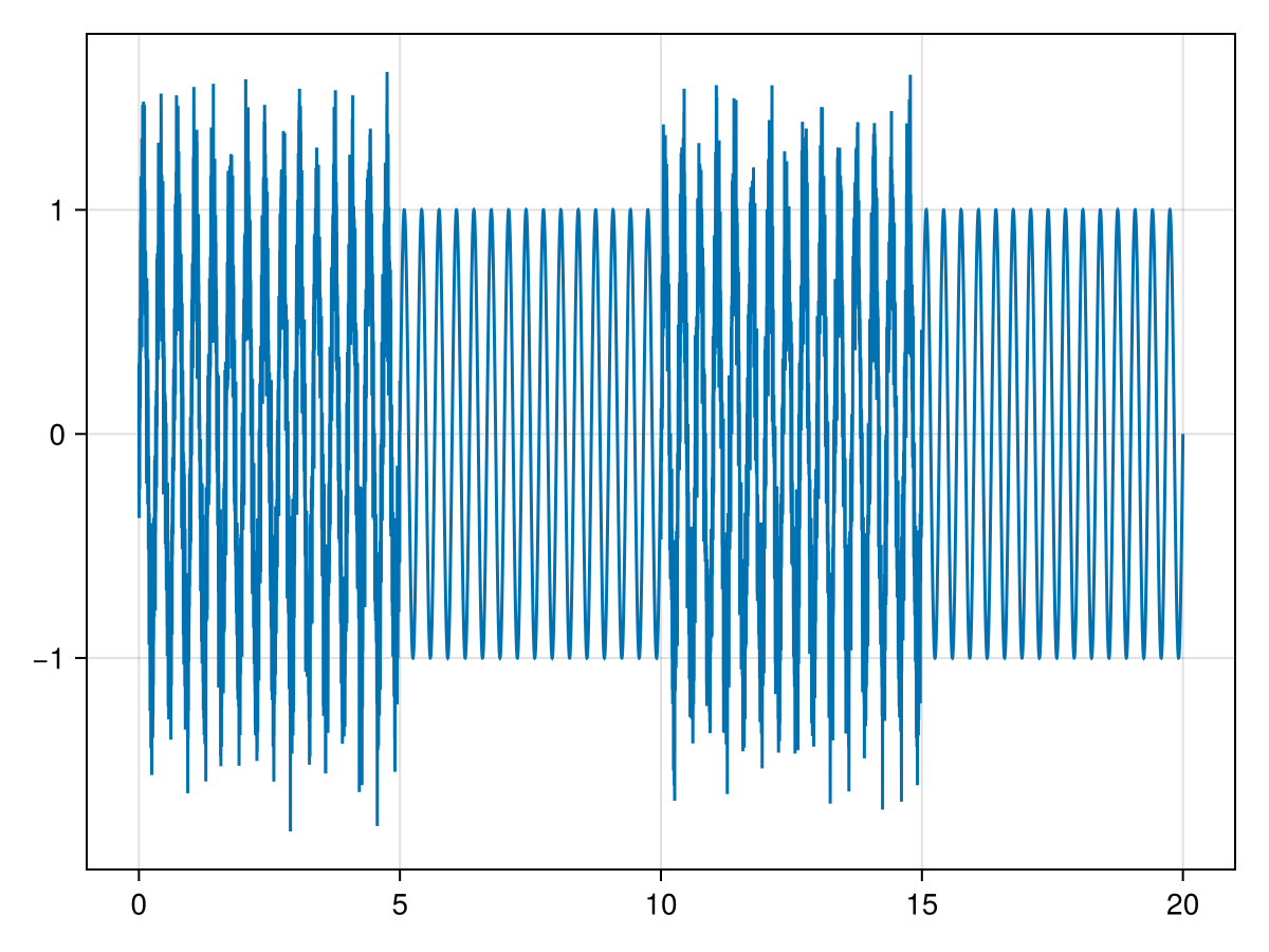
The disorder can be computed using the following method:
measure(settings::Disorder{N}, dataset::Vector{StateSpaceSet}, th_min::Float64, th_max::Float64)To apply it, the time series must first be split into a vector of StateSpaceSet objects:
windows = [ data[(i + 1):(i + window_len)] for i in 0:window_len:(length(data) - window_len)]
dataset = Vector{StateSpaceSet}(undef, length(windows))
for i ∈ eachindex(windows)
    dataset[i] = StateSpaceSet(windows[i])
end

dataset
20-element Vector{StateSpaceSet}:
1-dimensional StateSpaceSet{Float64} with 500 points
1-dimensional StateSpaceSet{Float64} with 500 points
1-dimensional StateSpaceSet{Float64} with 500 points
1-dimensional StateSpaceSet{Float64} with 500 points
1-dimensional StateSpaceSet{Float64} with 500 points
1-dimensional StateSpaceSet{Float64} with 500 points
1-dimensional StateSpaceSet{Float64} with 500 points
1-dimensional StateSpaceSet{Float64} with 500 points
1-dimensional StateSpaceSet{Float64} with 500 points
1-dimensional StateSpaceSet{Float64} with 500 points
1-dimensional StateSpaceSet{Float64} with 500 points
1-dimensional StateSpaceSet{Float64} with 500 points
1-dimensional StateSpaceSet{Float64} with 500 points
1-dimensional StateSpaceSet{Float64} with 500 points
1-dimensional StateSpaceSet{Float64} with 500 points
1-dimensional StateSpaceSet{Float64} with 500 points
1-dimensional StateSpaceSet{Float64} with 500 points
1-dimensional StateSpaceSet{Float64} with 500 points
1-dimensional StateSpaceSet{Float64} with 500 points
1-dimensional StateSpaceSet{Float64} with 500 pointsNext, the threshold range th_min and th_max must be defined. There are two possible approaches:
Use the full range of admissible threshold values by setting
th_min = 0andth_max = maximum(pairwise(Euclidean(), data, data)), and choosing a small step size via thenum_testskeywork argument (e.g.,num_tests = 1000). This approach yields the global maximum disorder values but can be computationally expensive.Use a small interval centered around a known threshold value. This is the recommended approach and is adopted here.
To obtain a suitable reference threshold, we select a subset of windows and compute the optimal disorder threshold using the optimize function:
using Statistics

function find_threshold(disorder, data)
    ths = zeros(Float64, 10)
    for i ∈ eachindex(ths)
        idx = rand(1:length(windows))
        ths[i] = optimize(Threshold(), disorder, data[idx])[1]
    end

    μ = mean(ths)
    σ = std(ths)

    return (max(0.0, μ - 1.5 * σ), μ + 1.5 * σ)
end
find_threshold (generic function with 1 method)dis = Disorder(4)
th_min, th_max = find_threshold(dis, dataset)(0.13274290497682428, 0.522905400201092)Finally, the disorder can be computed for all windows using the measure function:
results = measure(dis, dataset, th_min, th_max)20-element Vector{Float32}:
0.88537914
0.87818503
0.88202435
0.8803578
0.88093317
0.0817871
0.082624875
0.07967555
0.078830265
0.07897576
0.88101405
0.8840546
0.8756601
0.8731532
0.87767977
0.08167225
0.081700206
0.081684545
0.08164149
0.08268257scatterlines(results)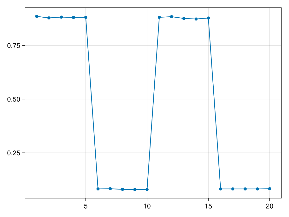
When computing Disorder for compatible time series, the same threshold range is used for all windows. However, the disorder value of each window corresponds to the maximum over that range, and therefore the optimal threshold may differ between windows.
Disorder can also be computed using the GPU backend:
measure(settings::Disorder{N}, dataset::Vector{<:AbstractGPUVector{SVector{D, Float32}}}, th_min::Float32, th_max::Float32)The procedure is identical, but each window must first be transferred to the GPU:
for i ∈ eachindex(windows)
    dataset[i] = StateSpaceSet(Float32.(windows[i])) |> CuVector
end