Examples

Only a few examples are shown here. Every method has an example (and plotting code) in the test folder!

Nonlinear

using SignalDecomposition, DynamicalSystems, Random, Plots, Statistics

he = Systems.henon()
tr = trajectory(he, 10000; Ttr = 100)
Random.seed!(151521)
z = tr[:, 1]
s = z .+ randn(10001)*0.1*std(z)
m = 5
metric = Euclidean()
k = 30
Q = [2, 2, 2, 3, 3, 3, 3]
x, r = decompose(s, ManifoldProjection(m, Q, k))
summary(x)

"10001-element Vector{Float64}"

p1 = plot(s, label = "input")
plot!(p1, z, color = :black, ls = :dash, label = "real")
plot!(p1, x, alpha = 0.5, label = "output")
xlims!(p1, 0, 50)
p1

Alright, this doesn't seem much of a difference to be honest. One sees a big difference once going into the state space and looking at the attractor:

p2 = scatter(s[1:end-1], s[2:end], ms = 1, label = "input", msw = 0)
scatter!(p2, z[1:end-1], z[2:end], ms = 1, label = "real", color = :black, msw = 0)
scatter!(p2, x[1:end-1], x[2:end], ms = 1, label = "output", alpha = 0.5, msw = 0)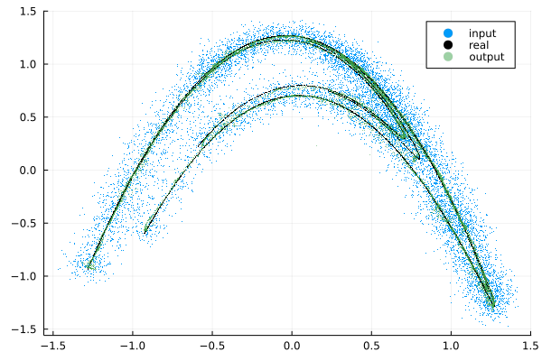

TimeAnomaly and Sinusoidal

using SignalDecomposition, Dates, Random, Plots
Random.seed!(41516)
y = Date(2001):Day(1):Date(2025)
dy = dayofyear.(y)
cy =  @. 4 + 7.2cos(2π*dy/365.26) + 5.6cos(4π*dy/365.26 + 3π/5)
r0 = randn(length(dy))/2
sy = cy .+ r0

x, r = decompose(y, sy, TimeAnomaly())

t = collect(1:length(y)) ./ 365.26 # true time in years

x2, r2 = decompose(t, sy, Sinusoidal([1.0, 2.0]))

p3 = plot(t, sy, label = "input")
plot!(p3, t, cy, label = "true periodic", color = :black, ls = :dash)
plot!(p3, t, x, label = "TimeAnomaly", alpha = 1.0, color = :red)
plot!(p3, t, x2, label = "Sinusoidal", alpha = 0.5, color = :green)
xlabel!(p3, "years")
xlims!(p3, 0, 1) # zoom in

Although not immediately obvious from the figure, Sinusoidal performs better:

rmse(cy, x), rmse(cy, x2)

(0.1200278668074404, 0.049766752176733646)

Furthermore, by construction, the x component of Sinusoidal will always be a smooth function (sum of cosines). TimeAnomaly will typically retain some noise.

Product

using SignalDecomposition, DynamicalSystems, Plots

ds = Systems.lorenz()
tr = trajectory(ds, 20; dt = 0.002, Ttr = 100)
lorenzx_slow = tr[:, 1]/std(tr[:, 1])

ds = Systems.roessler()
tr = trajectory(ds, 500.0, dt = 0.05, Ttr = 10)
roesslerz = tr[:, 3]/std(tr[:, 3])
roesslerz[roesslerz .≤ 0.1] .= 0

s = lorenzx_slow .* roesslerz
m = ProductInversion(roesslerz, 0.1:0.1:10)
x, r = decompose(s, m)

l = (4, 1)
p5 = plot(s, label = "input s")
plot!(p5, x .* r, label = "decomposed")
p6 = plot(lorenzx_slow, label = "original r")
plot!(p6, x, label = "decomposed r")
plot(p5, p6, layout=(2,1))