Phase Spaces
Coordinate Systems
Any billiard has two coordinate systems:
- The "real" coordinates, i.e. the coordinates that specify the full, three-dimensional phase space: $x, y, \phi$.
- The "boundary" coordinates, also known as Birkhoff coordinates, which instead reduce the continuous billiard into a map, by only considering the collision points. These coordinates are only two: $\xi, \sin(\phi_n)$, with $\xi$ being the parametrization of the arc length and $\phi_n$ being the angle as measured from the normal vector.
With DynamicalBilliards it is very easy to switch between the two coordinate systems, using:
DynamicalBilliards.to_bcoords — Functionto_bcoords(pos, vel, o::Obstacle) -> ξ, sφConvert the real coordinates pos, vel to boundary coordinates (also known as Birkhoff coordinates) ξ, sφ, assuming that pos is on the obstacle.
ξ is the arc-coordinate, i.e. it parameterizes the arclength of the obstacle. sφ is the sine of the angle between the velocity vector and the vector normal to the obstacle.
The arc-coordinate ξ is measured as:
- the distance from start point to end point in
Walls - the arc length measured counterclockwise from the open face in
Semicircles - the arc length measured counterclockwise from the rightmost point in
Circular/Ellipses
Notice that this function returns the local arclength. To get the global arclength parameterizing an entire billiard, simply do ξ += arcintervals(bd)[i] if the index of obstacle o is i.
See also from_bcoords, which is the inverse function.
DynamicalBilliards.from_bcoords — Functionfrom_bcoords(ξ, sφ, o::Obstacle) -> pos, velConvert the boundary coordinates ξ, sφ on the obstacle to real coordinates pos, vel.
Note that vel always points away from the obstacle.
This function is the inverse of to_bcoords.
from_bcoords(ξ, sφ, bd::Billiard, intervals = arcintervals(bd))Same as above, but now ξ is considered to be the global arclength, parameterizing the entire billiard, instead of a single obstacle.
DynamicalBilliards.arcintervals — Functionarcintervals(bd::Billiard) -> sGenerate a vector s, with entries being the delimiters of the arclengths of the obstacles of the billiard. The arclength from s[i] to s[i+1] is the arclength spanned by the ith obstacle.
s is used to transform an arc-coordinate ξ from local to global and vice-versa. A local ξ becomes global by adding s[i] (where i is the index of current obstacle). A global ξ becomes local by subtracting s[i].
See also boundarymap, to_bcoords, from_bcoords.
Boundary Maps
Boundary maps can be obtained with the high level function
DynamicalBilliards.boundarymap — Functionboundarymap(p, bd, t [,intervals]) → bmap, arclengthsCompute the boundary map of the particle p in the billiard bd by evolving the particle for total amount t (either float for time or integer for collision number).
Return a vector of 2-vectors bmap and also arclengths(bd). The first entry of each element of bmap is the arc-coordinate at collisions $\xi$, while the second is the sine of incidence angle $\sin(\phi_n)$.
The measurement direction of the arclengths of the individual obstacles is dictated by their order in bd. The sine of the angle is computed after specular reflection has taken place.
The returned values of this function can be used in conjuction with the function bdplot_boundarymap (requires using PyPlot) to plot the boundary map in an intuitive way.
Notice - this function only works for normal specular reflection. Random reflections or ray-splitting will give unexpected results.
See also to_bcoords, boundarymap_portion. See parallelize for a parallelized version.
For example, take a look at boundary maps of the mushroom billiard, which is known to have a mixed phase space:
using DynamicalBilliards, CairoMakie

bd = billiard_mushroom()

n = 100 # how many particles to create
t = 200 # how long to evolve each one

bmap, arcs = parallelize(boundarymap, bd, t, n)

randomcolor(args...) = RGBAf(0.9 .* (rand(), rand(), rand())..., 0.75)

colors = [randomcolor() for i in 1:n] # random colors

fig, ax = bdplot_boundarymap(bmap, arcs; color = colors)
fig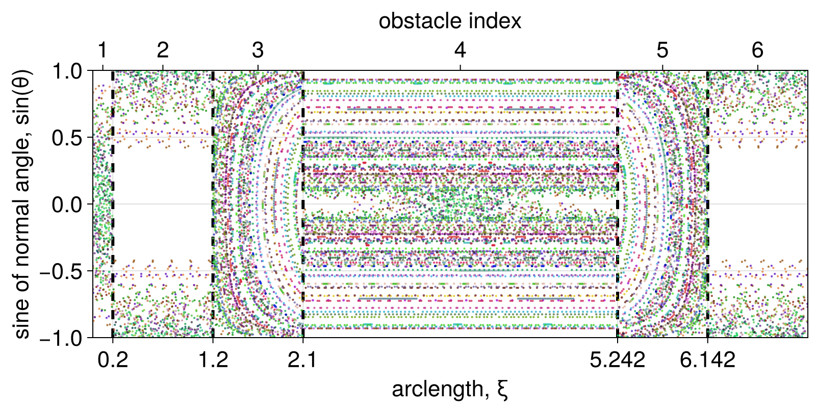
Phase Space Portions
It is possible to compute the portion of phase space covered by a particle as it is evolved in time. We have two methods, one for the "boundary" coordinates (2D space) and one for the "real" coordinates (3D space):
DynamicalBilliards.boundarymap_portion — Functionboundarymap_portion(bd::Billiard, t, p::AbstractParticle, δξ, δφ = δξ)Calculate the portion of the boundary map of the billiard bd covered by the particle p when it is evolved for time t (float or integer). Notice that the
The boundary map is partitioned into boxes of size (δξ, δφ) and as the particle evolves visited boxes are counted. The returned ratio is this count divided by the total boxes of size (δξ, δφ) needed to cover the boundary map.
Important: This portion does not equate the portion the particle's orbit covers on the full, three dimensional phase space. Use the function phasespace_portion for that!
DynamicalBilliards.phasespace_portion — Functionphasespace_portion(bd::Billiard, t, p::AbstractParticle, δξ, δφ = δξ)Calculate the portion of the phase space of the billiard bd covered by the particle p when it is evolved for time t (float or integer).
This function extends boundarymap_portion using a novel approach. For each visited box of the boundary map, bounce! attributes a third dimension (the collision time, equal to collision distance) which expands the two dimensions of the boundary map to the three dimensions of the phase space.
The true phase space portion is then the weighted portion of boxes visited by the particle, divided by the total weighted sum of boxes. The weights of the boxes are the collision times.
For example, for mushroom billiards the ratio of the chaotic-to-total phase space is known analytically for both the full 3D [1] space as well as the boundary 2D [2] space:
\[\begin{aligned} g_\text{c, 3D} &= \frac{2 \, \pi r^{2} - 4 \, r^{2} \arccos\left(\frac{w}{2 \, r}\right) + 4 \, l w + \sqrt{4 \, r^{2} - w^{2}} w}{2 \, {\left(\pi r^{2} + 2 \, l w\right)}}\\ g_\text{c, 2D} &= \frac{\pi w + 2 \, w \arccos\left(\frac{w}{2 \, r}\right) + 4 \, l + 4 \, r - 2 \, \sqrt{4 \, r^{2} - w^{2}}}{2 \, {\left(\pi r + 2 \, l + 2 \, r\right)}} \end{aligned}\]
We can easily confirm those formulas:
using DynamicalBilliards

t = 1000000.0
l = 1.0; r = 1.0; w = 0.4

bd = billiard_mushroom(l, w, r)

p = MushroomTools.randomchaotic(l, w, r)

ratio, dic = boundarymap_portion(bd, t, p, 0.01)
trueratio = MushroomTools.g_c_2D(l,w,r)
println("2D numeric - theory: $(abs(ratio - trueratio))")

ratio = phasespace_portion(bd, t, p, 0.01)
trueratio = MushroomTools.g_c_3D(l,w,r)
println("3D numeric - theory: $(abs(ratio - trueratio))")
2D numeric - theory: 0.0028617225371849186
3D numeric - theory: 0.00044067994432689384Of course, increasing evolution time and decreasing boxsize will bring higher accuracy.
References
[1] : A. H. Barnett & T. Betcke, Quantum mushroom billiards, Chaos, 17(4) (20017)
[2] : Lukas Hupe, B.Sc. Thesis (2018), to be published