Ray-Splitting

Ray-splitting is a semi-classical approach to the billiard system, giving a wave attribute to the ray traced by the particle. Upon collision a particle may propagate through an obstacle (transmission & refraction) or be reflected. Following the mindset of this package, implementing a ray-splitting billiard requires only three simple steps. We will introduce them and demonstrate them using a simple example in this documentation page.

1. Ray-Splitting Obstacles

The first step is that an Obstacle that supports ray-splitting is required to be present in your billiard table. The only new feature these obstacles have is an additional Boolean field called pflag (propagation flag). This field notes on which side of the obstacle the particle is currently propagating.

The normal vector as well as the distance from boundary change sign depending on the value of pflag. The obstacles Antidot, SplitterWall and FiniteSplitterWall are the equivalents of disk, wall and finite-wall for ray-splitting.

Let's create a billiard with a bunch of ray-splitting obstacles!

using DynamicalBilliards
x, y = 2.0, 1.0
bdr =  billiard_rectangle(x, y)
sw = SplitterWall([x/2, 0.0], [x/2,y], [-1,0], true)
a1 = Antidot([x/4, y/2], 0.25, "Left Antidot")
a2 = Antidot([3x/4, y/2], 0.15, "Right Antidot")
bd = Billiard(a1, a2, sw, bdr...)

Billiard{Float64} with 7 obstacles:
  Left Antidot
  Right Antidot
  Splitter wall
  Bottom wall
  Right wall
  Top wall
  Left wall

using InteractiveDynamics, CairoMakie
fig, ax = bdplot(bd)
fig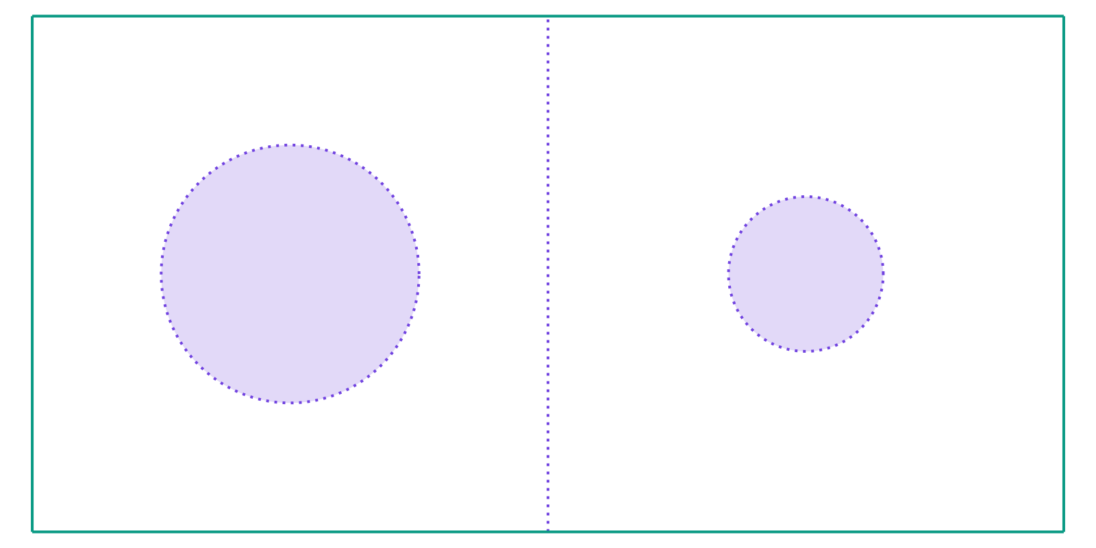

(notice also that raysplitting obstacles are by default plotted with a different color and with dotted linestyle)

2. The RaySplitter structure

In the second step, you have to define 2+1 functions: transmission probability, refraction angle and optionally new angular velocity after transmission. These functions, as well as which obstacles participate in ray-splitting, are bundled into a special structure:

RaySplitter(idxs, transmission, refraction [, newangular]; affect)

If you want different type of transmission/refraction functions for different obstacles, then you define multiple RaySplitters.

Continuing from the above billiard, let's also create some RaySplitter instances for it.

First define a refraction function

refraction(φ, pflag, ω) = pflag ? 0.5φ : 2.0φ

refraction (generic function with 1 method)

Then, a transmission probability function. In this example, we want to create a function that given some factor p, it returns a probability weighted with p in one direction of ray-splitting and 1-p in another direction.

transmission_p(p) = (φ, pflag, ω) -> begin
    if pflag
        p*exp(-(φ)^2/2(π/8)^2)
    else
        abs(φ) < π/4 ? (1-p)*exp(-(φ)^2/2(π/4)^2) : 0.0
    end
end

transmission_p (generic function with 1 method)

Notice also how we defined the function in such a way that critical refraction is respected, i.e. if θ(φ) ≥ π/2 then T(φ) = 0. Although this is necessary from a physical perspective, the code does take care of it by clamping the refraction angle (see below).

Lastly, for this example we will use magnetic propagation. We define functions such that the antidots also reverse the direction and magnitude of the magnetic field.

newoantidot(x, bool) =  bool ? -2.0x : -0.5x
newowall(x, bool) = bool ? 0.5x : 2.0x

newowall (generic function with 1 method)

Now we create the RaySplitter instances we want

raywall = RaySplitter([3], transmission_p(0.5), refraction, newowall)
raya = RaySplitter([1, 2], transmission_p(0.8), refraction, newoantidot)

RaySplitter for indices [1, 2]
 transmission: #1
 refraction:   refraction
 new angular:  newoantidot
 affect:       default

Because we want to use same functions for both antidots, we gave both indices in raya, [1, 2] (which are the indices of the antidots in the billiard bd).

3. Evolution with Ray-Splitting

The third step is trivial. After you have created your RaySplitter(s), you simply pass them into evolve or timeseries as a fourth argument! If you have many instances of RaySplitter you pass a tuple of them.

For example,

using Random, InteractiveDynamics, CairoMakie
Random.seed!(42)
p = randominside(bd, 1.0)
raysplitters = (raywall, raya)
xt, yt, vxt, vyt, tt = timeseries(p, bd, 100, raysplitters)
fig, ax = bdplot(bd)
lines!(ax, xt, yt)
scatter!(ax, xt[[1, 100]], yt[[1, 100]]; color = "black")
fig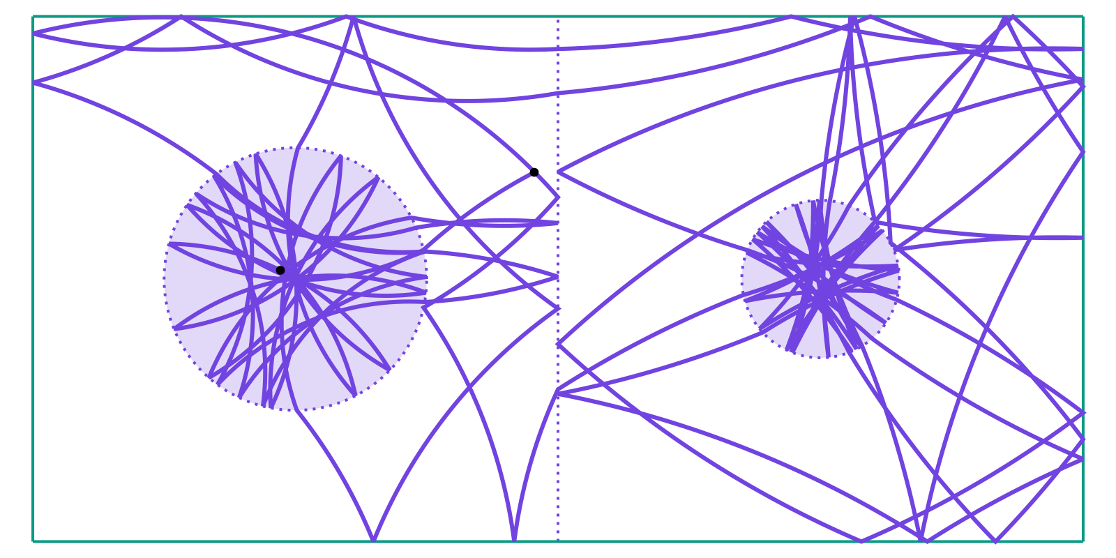

You can see that at some points the particle crossed the boundaries of the red obstacles, which allow for ray splitting.

The Ray-Splitting Algorithm

In this section we describe the algorithm we follow to implement the ray-splitting process. Let $T$ denote the transmission function, $\theta$ the refraction function and $\omega_{\text{new}}$ the new angular velocity function. The following describes the process after a particle has reached an obstacle that supports ray-splitting.

1. Find the angle of incidence $\phi' = \pi - \arccos(\vec{v} \cdot \vec{n}) = \arccos(\vec{v} \cdot (-\vec{n}))$ with $\vec{n}$ the normal vector at collision point. Notice that we use here $-\vec{n}$ because the velocity is opposing the normal vector before the collision happens. Using $-\vec{n}$ gives the angle between 0 and $\pi/2$ instead of $\pi/2$ to $\pi$.

2. Find the correct sign of the incidence angle, $\phi = \pm \phi'$. Specifically, use the cross product: if the third entry of $\vec{v} \times \vec{n}$ is negative, then have minus sign. The "correct" sign debates on whether the velocity vector is to the right or to the left of $(-\vec{n})$. This is important for finding the correct transmission angle and/or probability.

3. Check if $T(\phi, \verb|pflag|, \omega) > \text{random}()$. If not, do standard specular reflection.

4. If ray-splitting happens, then relocate the particle so that it is on the other side of the colliding obstacle. This contrasts the main evolution algorithm of this billiard package.

5. Re-compute the correct angle of incidence, as the position of the particle generally changes with relocating.

6. Find refraction angle $\theta(\phi, \verb|pflag|, \omega)$. Notice that this is a relative angle with respect to the normal vector. Also notice that $\theta$ may have opposite sign from $\phi$. It depends on the user if they want to add anomalous refraction.

7. Set obstacle.pflag = !obstacle.pflag for all obstacles affected by the current RaySplitter. This reverses $\vec{n}$ to $-\vec{n}$ as well! So from now on $\vec{n}$ is the opposite than what it was at the beginning of the algorithm!

8. Find the refraction angle in absolute space. First find $a = \text{atan}(n_y, n_x)$ and then set $\Theta = a + \theta$.

9. Perform refraction, i.e. set the particle velocity to the direction of $\Theta$.

10. Scale the magnetic field, i.e. set p.omega = $\omega_{\text{new}}(\omega, \verb|!pflag|)$. It is important to note that we use !pflag because we have already changed the pflag field.

Physics of the Ray-Splitting Functions

If T is the transmission probability function, then the condition for transmission is simply: T(φ, pflag, ω) > rand(). If it returns true, transmission (i.e. ray-splitting) will happen.

The functions given to RaySplitter should have some properties in order to have physical meaning. In order to test if the RaySplitter you have defined has physical meaning, the function isphysical is provided

isphysical(raysplitter(s))

Snell's Law

In classical geometric optics, the refraction of a ray of light moving from one medium to another is described by Snell's law. For an angle of incidence of $\phi$, the refraction angle $\theta$ is determined by the equation

where $n$ and $n'$ are the respective refractive indices of the media.

To easily simulate these relations in DynamicalBilliards, the function law_of_refraction can be used to set up ray-splitting according to this law.

law_of_refraction(n1, n2 = 1.0) -> t, r

Animation of Inverse Billiards

Here we will show an application of inverse billiards, where particles go in and out of a billiard, while taking advantage of the existence of a strong magnetic field outside of the billiard to return.

As always, we define the ray-splitting functions:

using DynamicalBilliards
trans(args...) = 1.0 # always perfect transmission
refra(φ, pflag, ω) = pflag ? 0.8φ : 1.25φ # refraction angle
neww(ω, pflag) = pflag ? 2.0 : 0.4

neww (generic function with 1 method)

Now, when we define the RaySplitter instance we will choose a different value for affect:

ray = RaySplitter([1,2,3,4], trans, refra, neww, affect = (i) -> SVector(1,2,3,4))

RaySplitter for indices [1, 2, 3, 4]
 transmission: trans
 refraction:   refra
 new angular:  neww
 affect:       #3

We initialize a simple rectangular billiard and a particle

bd = billiard_rectangle(setting = "ray-splitting")
p = MagneticParticle(0.4, 0.6, 0.0, 0.4)

MagneticParticle{Float64}
position: [0.4, 0.6]
velocity: [1.0, 0.0]
ang. velocity: 0.4

bdplot_interactive does not accept ray-splitters yet (but it is easy if you want to do a PR). Nevertheless, doing an animation is still straightforward:

using InteractiveDynamics, CairoMakie

fig, ax = bdplot(bd)
xlims!(ax, (-1, 2)); ylims!(ax, (-1, 2)) # zoom out
xt, yt = timeseries(p, bd, 10.0, (ray,))
D = 300
xta = Observable(xt[1:D])
yta = Observable(yt[1:D])
lines!(ax, xta, yta; color = :green)

record(fig, "inverse_billiard.mp4", D+1:length(xt); framerate = 30) do i
    push!(xta[], xt[i]); popfirst!(xta[])
    push!(yta[], yt[i]); popfirst!(yta[])
    notify.((xta, yta))
end