Lyapunov Exponents

The Finite Time Lyapunov Spectrum (FTLS) for a 2D billiard system consists of a set of 4 numbers $\lambda_i \, , \{ i = 1, ...,4 \}$ that characterize how fast the separation of initially close initial conditions grows.

It can be shown theoretically that two of these exponents must be zero ($\lambda_2$ =$\lambda_3$ = 0) and the other two are paired in such a way that they sum up to zero, i.e. $\lambda_1 = -\lambda_4$).

The function provided to calculate the FTLS is

DynamicalBilliards.lyapunovspectrum — Function

lyapunovspectrum([p::AbstractParticle,] bd::Billiard, t)

Returns the finite time lyapunov exponents (averaged over time t) for a given particle in a billiard table using the method outlined in [1]. t can be either Float or Int, meaning total time or total amount of collisions.

Returns zeros for pinned particles.

If a particle is not given, a random one is picked through randominside. See parallelize for a parallelized version.

[1] : Ch. Dellago et al, Phys. Rev. E 53 (1996)

source

Here its basic use is illustrated

using DynamicalBilliards

radius = 1.0
l = 2.0

bd = Billiard(billiard_polygon(6, l; setting = "periodic")..., Disk([0., 0.], radius))

par = randominside(bd)
t = 1000.0

exps = lyapunovspectrum(par, bd, t)

4-element Vector{Float64}:
  0.49039448921002976
  0.0018132739785905656
 -1.3480427061826369e-5
 -0.4921942827615574

In the following example we compute the change of $\lambda_1\$ versus the distance between the disks in a hexagonal periodic billiard.

using DynamicalBilliards, CairoMakie

t = 5000.0
radius = 1.0

spaces = 2.0:0.1:4.4 #Distances between adjacent disks
lyap_time = zero(spaces) #Array where the exponents will be stored

for (i, space) in enumerate(spaces)
    bd = billiard_polygon(6, space/(sqrt(3)); setting = "periodic")
    disc = Disk([0., 0.], radius)
    billiard = Billiard(bd.obstacles..., disc)
    p = randominside(billiard)
    lyap_time[i] = lyapunovspectrum(p, billiard, t)[1]
end
fig = Figure(); ax = Axis(fig[1,1]; xlabel = L"w" ylabel = L"\lambda_1")
lines!(ax,spaces, lyap_time)
fig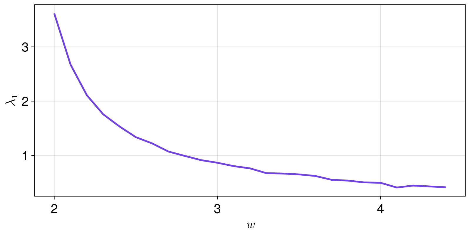

┌ Warning: Assignment to `bd` in soft scope is ambiguous because a global variable by the same name exists: `bd` will be treated as a new local. Disambiguate by using `local bd` to suppress this warning or `global bd` to assign to the existing global variable.
└ @ none:3

The plot of the maximum exponent can be compared with the results reported by Gaspard et. al (see figure 7), showing that using just t = 5000.0 is already enough of a statistical averaging.

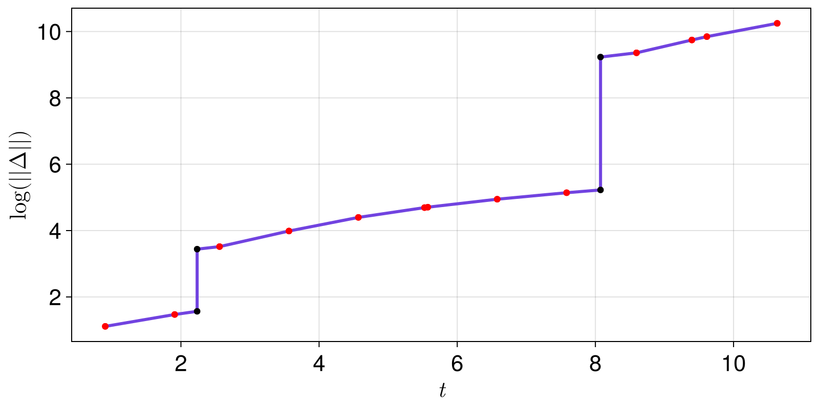
Perturbation Growth

To be able to inspect the dynamics of perturbation growth in more detail, we also provide the following function:

DynamicalBilliards.perturbationgrowth — Function

perturbationgrowth([p,] bd, t) -> ts, Rs, is

Calculate the evolution of the perturbation vector Δ along the trajectory of p in bd for total time t. Δ is initialised as [1,1,1,1].

If a particle is not given, a random one is picked through randominside. Returns empty lists for pinned particles.

Description

This function safely computes the time evolution of a perturbation vector using the linearized dynamics of the system, as outlined by [1]. Because the dynamics are linear, we can safely re-normalize the perturbation vector after every collision (otherwise the perturbations grow to infinity).

Immediately before and after every collison, this function computes

the current time.
the element-wise ratio of Δ with its previous value
the obstacle index of the current obstacle

and returns these in three vectors ts, Rs, is.

To obtain the actual evolution of the perturbation vector you can use the function perturbationevolution(Rs) which simply does

Δ = Vector{SVector{4,Float64}}(undef, length(R))
Δ[1] = R[1]
for i in 2:length(R)
    Δ[i] = R[i] .* Δ[i-1]
end

[1] : Ch. Dellago et al, Phys. Rev. E 53 (1996)

source

For example, lets plot the evolution of the perturbation growth using different colors for collisions with walls and disks in the Sinai billiard:

using DynamicalBilliards, CairoMakie, LinearAlgebra
bd = billiard_sinai()

ts, Rs, is = perturbationgrowth(Particle(0.1, 0.1, 0.1), bd, 10.0)
Δ = perturbationevolution(Rs)

fig = Figure(); ax = Axis(fig[1,1]; xlabel = L"t", ylabel = L"\log(||\Delta ||)"))
lines!(ts, log.(norm.(Δ)))
scatter!(ts, log.(norm.(Δ)); color = [j == 1 ? :black : :red for j in is])
fig

30-element Vector{SVector{4, Float64}}:
 [1.9045188265604098, 1.9045188265604098, 1.0, 1.0]
 [-1.9045188265604098, 1.9045188265604098, -1.0, 1.0]
 [-2.909539744960865, 2.909539744960865, -1.0, 1.0]
 [2.909539744960865, 2.909539744960865, 1.0, 1.0]
 [3.234529363008706, 3.234529363008706, 1.0, 1.0]
 [-3.2293045272097873, -3.239745772568178, -30.794093877141325, 1.9393625284964386]
 [-13.22662898970294, -2.6101303493921058, -30.794093877141325, 1.9393625284964386]
 [-13.22662898970294, 2.6101303493921058, -30.794093877141325, -1.9393625284964386]
 [-44.170366682585126, 0.6613434939443076, -30.794093877141325, -1.9393625284964386]
 [-44.170366682585126, -0.6613434939443076, -30.794093877141325, 1.9393625284964386]
 ⋮
 [-181.54444103960654, 24.869529653403607, -10019.825390600476, 1929.9082905737866]
 [-5400.952886278822, 1030.174436444233, -10019.825390600476, 1929.9082905737866]
 [-5400.952886278822, -1030.174436444233, -10019.825390600476, -1929.9082905737866]
 [-13432.612657552925, -2577.144186455109, -10019.825390600476, -1929.9082905737866]
 [13432.612657552925, -2577.144186455109, 10019.825390600476, -1929.9082905737866]
 [15605.155537387785, -2995.5954420382236, 10019.825390600476, -1929.9082905737866]
 [15605.155537387785, 2995.5954420382236, 10019.825390600476, 1929.9082905737866]
 [25809.35818849675, 4961.016447632214, 10019.825390600476, 1929.9082905737866]
 [25809.35818849675, -4961.016447632214, 10019.825390600476, -1929.9082905737866]