Entropies and Dimensions

Generalized Entropy

In the study of dynamical systems there are many quantities that identify as "entropy". Notice that these quantities are not the more commonly known thermodynamic ones, used in Statistical Physics. Rather, they are more like the to the entropies of information theory, which represents information contained within a dataset, or information about the dimensional scaling of a dataset.

The main way of computing entropies in DynamicalSystems.jl is the "generalized entropy":

#ChaosTools.genentropy — Function.

genentropy(α, ε, dataset::AbstractDataset; base = e)

Compute the α order generalized (Rényi) entropy [1] of a dataset, by first partitioning it into boxes of length ε using non0hist.

genentropy(α, p::AbstractArray; base = e)

Compute the entropy of an array p directly, assuming that p is sum-normalized.

Optionally use base for the logarithms.

Description

Let $p$ be an array of probabilities (summing to 1). Then the Rényi entropy is

and generalizes other known entropies, like e.g. the information entropy ($\alpha = 1$, see [2]), the maximum entropy ($\alpha=0$, also known as Hartley entropy), or the correlation entropy ($\alpha = 2$, also known as collision entropy).

References

[1] : A. Rényi, Proceedings of the fourth Berkeley Symposium on Mathematics, Statistics and Probability, pp 547 (1960)

[2] : C. E. Shannon, Bell Systems Technical Journal 27, pp 379 (1948)

Basically, given a dataset you can partition it into boxes to calculate an entropy. See below for a detailed example.

The function used internally by genentropy is non0hist:

#ChaosTools.non0hist — Function.

non0hist(ε, dataset::AbstractDataset)

Partition a dataset into tabulated intervals (boxes) of size ε and return the sum-normalized histogram in an unordered 1D form, discarding all zero elements and bin edge information.

Performances Notes

This method has a linearithmic time complexity (n log(n) for n = length(data)) and a linear space complexity (l for l = dimension(data)). This allows computation of entropies of high-dimensional datasets and with small box sizes ε without memory overflow.

Use e.g. fit(Histogram, ...) from StatsBase if you wish to keep information about the edges of the binning as well as the zero elements.

Attractor Dimension Estimation

There are numerous methods that one can use to calculate a so-called "dimension" of a dataset, like for example the Fractal dimension. This real number can offer a lot of information about the object that the dataset represents.

Based on the definition of the generalized entropy, one can calculate an appropriate dimension, called generalized dimension:

#ChaosTools.generalized_dim — Function.

generalized_dim(α, dataset [, sizes]) -> D_α

Return the α order generalized dimension of the dataset, by calculating the genentropy for each ε ∈ sizes.

Description

The returned dimension is approximated by the (inverse) power law exponent of the scaling of the genentropy versus the box size ε, where ε ∈ sizes.

Calling this function performs a lot of automated steps:

1. A vector of box sizes is decided by calling sizes = estimate_boxsizes(dataset), if sizes is not given.
2. For each element of sizes the appropriate entropy is calculated, through d = genentropy.(α, sizes, dataset). Let x = -log.(sizes).
3. The curve d(x) is decomposed into linear regions, using linear_regions(x, d).
4. The biggest linear region is chosen, and a fit for the slope of that region is performed using the function linear_region. This slope is the return value of generalized_dim.

By doing these steps one by one yourself, you can adjust the keyword arguments given to each of these function calls, refining the accuracy of the result.

The following aliases are provided:

• α = 0 : boxcounting_dim, capacity_dim
• α = 1 : information_dim

#ChaosTools.estimate_boxsizes — Function.

estimate_boxsizes(dataset::AbstractDataset; k::Int = 12, z = -1, w = 1)

Return k exponentially spaced values: 10 .^ range(lower+w, upper+z, length = k).

lower is the magnitude of the minimum pair-wise distance between datapoints while upper is the magnitude of the maximum difference between greatest and smallest number among each timeseries.

"Magnitude" here stands for order of magnitude, i.e. round(log10(x)).

#ChaosTools.linear_regions — Function.

linear_regions(x, y; dxi::Int = 1, tol = 0.2) -> (lrs, tangents)

Identify regions where the curve y(x) is linear, by scanning the x-axis every dxi indices (e.g. at x[1] to x[5], x[5] to x[10], x[10] to x[15] and so on if dxi=5).

If the slope (calculated using LsqFit) of a region of width dxi is approximatelly equal to that of the previous region, within tolerance tol, then these two regions belong to the same linear region.

Return the indices of x that correspond to linear regions, lrs, and the approximated tangents at each region. lrs is a vector of Int. Notice that tangents is not accurate: it is not recomputed at every step, but only when its error exceeds the tolerance tol! Use linear_region to obtain a correct estimate for the slope of the largest linear region.

#ChaosTools.linear_region — Function.

linear_region(x, y; dxi::Int = 1, tol = 0.2) -> ([ind1, ind2], slope)

Call linear_regions, identify the largest linear region and approximate the slope of the entire region using linreg. Return the indices where the region starts and stops (x[ind1:ind2]) as well as the approximated slope.

Example

For an example of using entropies to compute the dimension of an attractor let's use everyone's favorite system:

using DynamicalSystems, PyPlot
lor = Systems.lorenz()

3-dimensional continuous dynamical system
 state:       [0.0, 10.0, 0.0]
 e.o.m.:      loop
 in-place?    false
 jacobian:    loop_jac
 parameters:  [10.0, 28.0, 2.66667]

Our goal is to compute entropies for many different partition sizes ε, so let's get down to it:

tr = trajectory(lor, 100.0; Ttr = 10.0)

ες = ℯ .^ (-3.5:0.5:3.5) # semi-random guess
Hs = genentropy.(1, ες, Ref(tr))

15-element Array{Float64,1}:
 9.203093741524961 
 9.192836189007936 
 9.175263277513562 
 9.11505930200447  
 8.96800482792302  
 8.650506643435117 
 8.093472893003044 
 7.329635456822501 
 6.440181060621013 
 5.520699459712151 
 4.5223766061173905
 3.5423893065177388
 2.688046235608927 
 1.9474099557575748
 0.8398578086498265

xs = @. -log(ες)
figure()
plot(xs, Hs)
ylabel("\$H_1\$")
xlabel("\$-\\log (\\epsilon)\$");

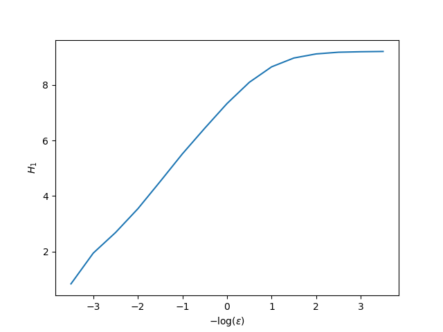
The slope of the linear scaling region of the above plot is the generalized dimension (of order α = 2) for the attractor of the Lorenz system.

Given that we see the plot, we can estimate where the linear scaling region starts and ends. However, we can use the function linear_region to get an estimate of the result as well. First let's visualize what it does:

lrs, slopes = linear_regions(xs, Hs, tol = 0.25)

figure()
for i in 1:length(lrs)-1
    plot(xs[lrs[i]:lrs[i+1]], Hs[lrs[i]:lrs[i+1]], marker = "o")
end
ylabel("\$H_1\$")
xlabel("\$-\\log (\\epsilon)\$");

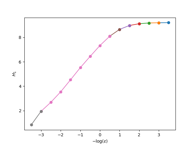
The linear_region function computes the slope of the largest region:

linear_region(xs, Hs)[2]

1.721554939214834

This result is an approximation of the information dimension (because we used α = 1) of the Lorenz attractor.

The above pipeline is bundled in generalized_dim. For example, the dimension of the strange attractor of the Hénon map, following the above approach but taking automated steps, is:

using DynamicalSystems
hen = Systems.henon()
ts = trajectory(hen, 200000)
D_hen = generalized_dim(1, ts)

1.215884931528749

As a side note, be sure that you have enough data points, otherwise the values you will get will never be correct, as is demonstrated by J.-P. Eckmann and D. Ruelle (see Physica D 56, pp 185-187 (1992)).

Other Entropies and Dimensions

Permutation Entropy

The permutation entropy is introduced by C. Bandt and B. Pompe as a "A Natural Complexity Measure for Timeseries", which directly applies to arbitrary real-world data and is particularly useful in the presence of dynamical or observational noise.

#ChaosTools.permentropy — Function.

permentropy(x::AbstractVector, order [, interval=1]; base = e)

Compute the permutation entropy [1] of given order from the x timeseries.

Optionally, interval can be specified to use x[t0:interval:t1] when calculating permutation of the sliding windows between t0 and t1 = t0 + interval * (order - 1).

Optionally use base for the logarithms.

References

[1] : C. Bandt, & B. Pompe, Phys. Rev. Lett. 88 (17), pp 174102 (2002)

For example, we will compute and compare the lyapunov exponent of the logistic map with the order-6 permutation entropy, like in the original paper.

using DynamicalSystems, PyPlot
ds = Systems.logistic()
rs = 3.5:0.001:4
ls = Float64[]; hs = Float64[]
for r in rs
    ds.p[1] = r
    push!(ls, lyapunov(ds, 100000))
    # For 1D systems `trajectory` returns a vector
    push!(hs, permentropy(trajectory(ds, 10000), 6))
end

f = figure(figsize = (10,6))
a1 = subplot(211)
plot(rs, ls); ylim(-2, log(2)); ylabel("\$\\lambda\$")
a1.axes.get_xaxis().set_ticklabels([])
xlim(rs[1], rs[end]);

a2 = subplot(212)
plot(rs, hs; color = "C1"); ylabel("\$h_6\$")
xlim(rs[1], rs[end]); xlabel("\$r\$")
tight_layout()

Kaplan-Yorke Dimension

#ChaosTools.kaplanyorke_dim — Function.

kaplanyorke_dim(lyapunovs::AbstractVector)

Calculate the Kaplan-Yorke dimension, a.k.a. Lyapunov dimension [1].

Description

The Kaplan-Yorke dimension is simply the point where cumsum(lyapunovs) becomes zero (interpolated). If the sum of the exponents never becomes negative the function will return the length of the input vector.

Useful in combination with lyapunovs.

References

[1] : J. Kaplan & J. Yorke, Chaotic behavior of multidimensional difference equations, Lecture Notes in Mathematics vol. 730, Springer (1979)

Notice that calling this function requires you to pass the Lyapunov exponents in an ordered vector form (largest to smallest). Example:

using DynamicalSystems
hen = Systems.henon()
D_kp = kaplanyorke_dim(lyapunovs(hen, 100000))

1.258697711464614