Nonlinear Timeseries Analysis

Numerical Lyapunov Exponent

Given any timeseries, one can first reconstruct it using delay coordinates, and then calculate a maximum Lyapunov exponent for it. This is done with

#ChaosTools.numericallyapunov — Function.

numericallyapunov(R::Dataset, ks;  refstates, w, distance, ntype)

Return E = [E(k) for k ∈ ks], where E(k) is the average logarithmic distance between states of a neighborhood that are evolved in time for k steps (k must be integer).

Keyword Arguments

• refstates = 1:(length(R) - ks[end]) : Vector of indices that notes which states of the reconstruction should be used as "reference states", which means that the algorithm is applied for all state indices contained in refstates.
• w::Int = 1 : The Theiler window, which determines whether points are separated enough in time to be considered separate trajectories (see [1] and neighborhood).
• ntype::AbstractNeighborhood = FixedMassNeighborhood(1) : The method to be used when evaluating the neighborhood of each reference state. See AbstractNeighborhood or neighborhood for more info.
• distance::Metric = Cityblock() : The distance function used in the logarithmic distance of nearby states. The allowed distances are Cityblock() and Euclidean(). See below for more info.

Description

If the dataset/reconstruction exhibits exponential divergence of nearby states, then it should clearly hold

for a well defined region in the k axis, where $\lambda$ is the approximated maximum Lyapunov exponent. $\Delta t$ is the time between samples in the original timeseries. You can use linear_region with arguments (ks .* Δt, E) to identify the slope (= $\lambda$) immediatelly, assuming you have choosen sufficiently good ks such that the linear scaling region is bigger than the saturated region.

The algorithm used in this function is due to Parlitz [1], which itself expands upon Kantz [2]. In sort, for each reference state a neighborhood is evaluated. Then, for each point in this neighborhood, the logarithmic distance between reference state and neighborhood state is calculated as the "time" index k increases. The average of the above over all neighborhood states over all reference states is the returned result.

If the Metric is Euclidean() then use the Euclidean distance of the full D-dimensional points (distance $d_E$ in ref. [1]). If however the Metric is Cityblock(), calculate the absolute distance of only the first elements of the m+k and n+k points of the reconstruction R (distance $d_F$ in ref. [1]).

References

[1] : Skokos, C. H. et al., Chaos Detection and Predictability - Chapter 1 (section 1.3.2), Lecture Notes in Physics 915, Springer (2016)

[2] : Kantz, H., Phys. Lett. A 185, pp 77–87 (1994)

The function numericallyapunov has a total of 4 different approaches for the algorithmic process, by combining 2 types of distances with 2 types of neighborhoods.

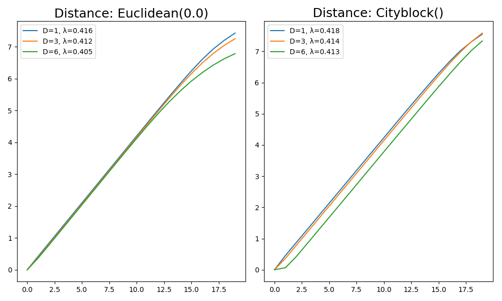
Example of Numerical Lyapunov computation

using DynamicalSystems, PyPlot

ds = Systems.henon()
data = trajectory(ds, 100000)
x = data[:, 1] #fake measurements for the win!

ks = 1:20
ℜ = 1:10000
fig = figure(figsize=(10,6))

for (i, di) in enumerate([Euclidean(), Cityblock()])
    subplot(1, 2, i)
    ntype = FixedMassNeighborhood(2)
    title("Distance: $(di)", size = 18)
    for D in [1, 3, 6]
        R = reconstruct(x, D, 1)
        E = numericallyapunov(R, ks;
        refstates = ℜ, distance = di, ntype = ntype)
        Δt = 1
        λ = linear_region(ks.*Δt, E)[2]
        # gives the linear slope, i.e. the Lyapunov exponent
        plot(ks .- 1, E .- E[1], label = "D=$D, λ=$(round(λ, digits = 3))")
        legend()
        tight_layout()
    end
end

Bad Time-axis (ks) length

Let's revisit the example of the previous section:

ds = Systems.henon()
data = trajectory(ds, 100000)
x = data[:, 1]
length(x)

100001

The timeseries of such length could be considered big. A time length of 100 seems very small. Yet it turns out it is way too big! The following

ks = 1:100
R = reconstruct(x, 1, 1)
E = numericallyapunov(R, ks, ntype = FixedMassNeighborhood(2))
figure()
plot(ks .- 1, E .- E[1])
title("Lyappunov: $(linear_region(ks, E)[2])")

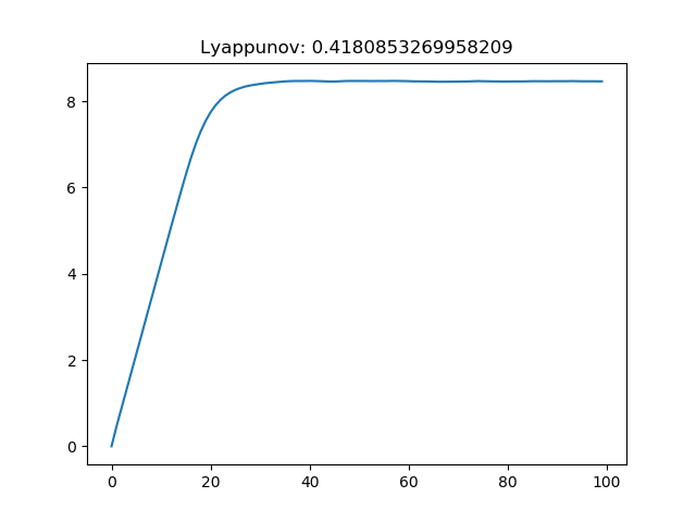
Notice that even though this value for the Lyapunov exponent is correct, it happened to be correct simply due to the jitter of the saturated region. Since the saturated region is much bigger than the linear scaling region, if it wasn't that jittery the function linear_region would not give the scaling of the linear region, but instead a slope near 0! (or if you were to give bigger tolerance as a keyword argument)

Case of a Continuous system

The process for continuous systems works identically with discrete, but one must be a bit more thoughtful when choosing parameters. The following example helps the users get familiar with the process:

using DynamicalSystems, PyPlot

ntype = FixedMassNeighborhood(5) #5 nearest neighbors of each state

ds = Systems.lorenz()
# create a timeseries of 1 dimension
dt = 0.05
x = trajectory(ds, 1000.0; dt = dt)[:, 1]

20001-element Array{Float64,1}:
  0.0               
  4.285178117517708 
  8.924780522479637 
 15.012203311102235 
 20.05533894475613  
 18.062350952804728 
  9.898343637398332 
  2.199113375749754 
 -2.6729722259323863
 -5.33812377718313  
  ⋮                 
  8.982259166809083 
 10.670302924424051 
 11.842660338013772 
 11.87017960987118  
 10.618810328221139 
  8.656181145701055 
  6.751870416569524 
  5.371698729920532 
  4.63198025969704  

We know that we have to use much bigger ks than 1:20, because this is a continuous case! (See reference given in numericallyapunovs)

ks1 = 0:200

0:200

and in fact it is even better to not increment the ks one by one but instead do

ks2 = 0:4:200

0:4:200

Now we plot some example computations

figure()
for D in [3, 7], τ in [7, 15]
    r = reconstruct(x, D, τ)

    # E1 = numericallyapunov(r, ks1; ntype = ntype)
    # λ1 = linear_region(ks1 .* dt, E1)[2]
    E2 = numericallyapunov(r, ks2; ntype = ntype)
    λ2 = linear_region(ks2 .* dt, E2)[2]

    # plot(ks1,E1.-E1[1], label = "dense, D=$(D), τ=$(τ), λ=$(round(λ1, 3))")
    plot(ks2,E2.-E2[1], label = "D=$(D), τ=$(τ), λ=$(round(λ2, digits = 3))")
end

legend()
xlabel("k (0.05×t)")
ylabel("E - E(0)")
title("Continuous Reconstruction Lyapunov")
tight_layout()

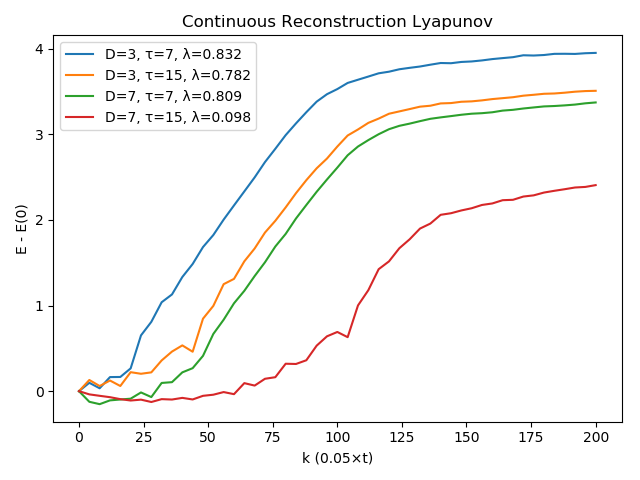
As you can see, using τ = 15 is not a great choice! The estimates with τ = 7 though are very good (the actual value is around λ ≈ 0.89...).

Broomhead-King Coordinates

#ChaosTools.broomhead_king — Function.

broomhead_king(s::AbstractVector, d::Int) -> U, S, Vtr

Return the Broomhead-King coordinates of a timeseries s by performing svd on the so-called trajectory matrix with dimension d.

Description

Broomhead and King coordinates is an approach proposed in [1] that applies the Karhunen–Loève theorem to delay coordinates embedding with smallest possible delay.

The function performs singular value decomposition on the d-dimensional trajectory matrix $X$ of $s$,

where $x := s - \bar{s}$. The columns of $U$ can then be used as a new coordinate system, and by considering the values of the singular values $S$ you can decide how many columns of $U$ are "important". See the documentation page for example application.

References

[1] : D. S. Broomhead, R. Jones and G. P. King, J. Phys. A 20, 9, pp L563 (1987)

This alternative/improvement of the traditional delay coordinates can be a very powerful tool. An example where it shines is noisy data where there is the effect of superficial dimensions due to noise.

Take the following example where we produce noisy data from a system and then use Broomhead-King coordinates as an alternative to "vanilla" delay coordinates:

using DynamicalSystems, PyPlot

ds = Systems.gissinger()
data = trajectory(ds, 1000.0, dt = 0.05)
x = data[:, 1]

L = length(x)
s = x .+ 0.5rand(L) #add noise

U, S = broomhead_king(s, 40)
summary(U)

"19962×40 Array{Float64,2}"

Now let's simply compare the above result with the one you get from doing a "standard" call to reconstruct:

figure(figsize= (10,6))
subplot(1,2,1)
plot(U[:, 1], U[:, 2])
title("Broomhead-King of s")

subplot(1,2,2)
R = reconstruct(s, 1, 30)
plot(columns(R)...; color = "C3")
title("2D reconstruction of s")
tight_layout()

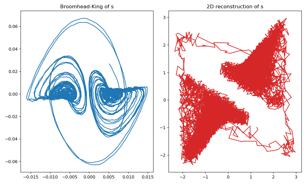
we have used the same system as in the delay coordinates reconstruction example, and picked the optimal delay time of τ = 30 (for same dt = 0.05). Regardless, the vanilla delay coordinates is much worse than the Broomhead-King coordinates.