Dansgaard-Oescher events and Critical Slowing Down

The $\delta^{18}O$ timeseries of the North Greenland Ice Core Project (NGRIP) are, to this date, the best proxy record for the Dansgaard-Oeschger events (DO-events). DO-events are sudden warming episodes of the North Atlantic, reaching 10 degrees of regional warming within 100 years. They happened quasi-periodically over the last glacial cycle due to transitions between strong and weak states of the Atlantic Meridional Overturning Circulation and might be therefore be the most prominent examples of abrupt transitions in the field of climate science. We here propose to hindcast these events by applying the theory of Critical Slowing Down (CSD) on the NGRIP data, which can be found here in its raw format. This analysis has already been done in (Boers, 2018) and we here try to reproduce Figure 2.d-f.

Preprocessing NGRIP

Data pre-processing is not part of TransitionsInTimeseries.jl, but a step the user has to do before using the package. To present an example with a complete scientific workflow, we will showcase typical data pre-processing here, that consist of the following steps:

1. Load the data, reverse and offset it to have time vector = time before 2000 AD.
2. Filter non-unique points in time and sort the data.
3. Regrid the data from uneven to even sampling.

The time and $\delta^{18}O$ vectors resulting from the $i$-th preprocessing step are respectively called $t_i$ and $x_i$. The final step consists in obtaining a residual $r$, i.e. the fluctuations of the system around the attractor, which, within the CSD theory, is assumed to be tracked. Over this example, it will appear that the convenience of TransitionsInTimeseries.jl leads the bulk of the code to be written for plotting and preprocessing.

Step 1:

using DelimitedFiles, Downloads

function load_ngrip()
    tmp = Base.download("https://raw.githubusercontent.com/JuliaDynamics/JuliaDynamics/"*
        "master/timeseries/NGRIP.csv")
    data, labels = readdlm(tmp, header = true)
    return reverse(data[:, 1]) .- 2000, reverse(data[:, 2]) # (time, delta-18-0) vectors
end

t1, x1 = load_ngrip()

([-59944.5, -59939.6, -59935.9, -59930.5, -59925.0, -59919.0, -59914.3, -59909.4, -59904.5, -59899.7  …  -27.40000000000009, -27.40000000000009, -27.299999999999955, -27.299999999999955, -27.200000000000045, -27.09999999999991, -27.09999999999991, -27.0, -26.90000000000009, -26.799999999999955], [-43.52, -42.94, -42.13, -40.04, -41.09, -43.57, -42.28, -41.2, -44.07, -44.53  …  -35.29, -35.18, -35.51, -36.03, -36.52, -37.12, -37.41, -37.21, -36.62, -35.52])

Step 2

uniqueidx(v) = unique(i -> v[i], eachindex(v))
function keep_unique(t, x)
    unique_idx = uniqueidx(t)
    return t[unique_idx], x[unique_idx]
end

function sort_timeseries!(t, x)
    p = sortperm(t)
    permute!(t, p)
    permute!(x, p)
    return nothing
end

t2, x2 = keep_unique(t1, x1)
sort_timeseries!(t2, x2)

Step 3

using BSplineKit

function regrid2evensampling(t, x, dt)
    itp = BSplineKit.interpolate(t, x, BSplineOrder(4))
    tspan = (ceil(minimum(t)), floor(maximum(t)))
    t_even = collect(tspan[1]:dt:tspan[2])
    x_even = itp.(t_even)
    return t_even, x_even
end

dt = 5.0        # dt = 5 yr as in (Boers 2018)
t3, x3 = regrid2evensampling(t2, x2, dt)

([-59944.0, -59939.0, -59934.0, -59929.0, -59924.0, -59919.0, -59914.0, -59909.0, -59904.0, -59899.0  …  -74.0, -69.0, -64.0, -59.0, -54.0, -49.0, -44.0, -39.0, -34.0, -29.0], [-43.445268010797946, -42.85408835164853, -41.357360665158936, -39.9365468206892, -41.60554051352076, -43.57000000000001, -42.145558689100454, -41.33160823883399, -44.273597725729985, -44.4622612304012  …  -35.12, -36.190000000000005, -35.14, -37.06, -34.93, -34.23, -33.53, -35.09, -34.00000000000001, -34.46])

Step 4

For the final step we drop the indices:

using DSP

function chebyshev_filter(t, x, fcutoff)
    ii = 10             # Chebyshev filtering requires to prune first points of timeseries.
    responsetype = Highpass(fcutoff, fs = 1/dt)
    designmethod = Chebyshev1(8, 0.05)
    r = filt(digitalfilter(responsetype, designmethod), x)
    xtrend = x - r
    return t[ii:end], x[ii:end], xtrend[ii:end], r[ii:end]
end

fcutoff = 0.95 * 0.01   # cutoff ≃ 0.01 yr^-1 as in (Boers 2018)
t, x, xtrend, r = chebyshev_filter(t3, x3, fcutoff)

([-59899.0, -59894.0, -59889.0, -59884.0, -59879.0, -59874.0, -59869.0, -59864.0, -59859.0, -59854.0  …  -74.0, -69.0, -64.0, -59.0, -54.0, -49.0, -44.0, -39.0, -34.0, -29.0], [-44.4622612304012, -44.264401428210874, -44.02956767939856, -42.29334237357212, -42.594341674200344, -41.09704877854712, -40.39837540966913, -44.369155046413255, -42.74492506508012, -43.737014520530145  …  -35.12, -36.190000000000005, -35.14, -37.06, -34.93, -34.23, -33.53, -35.09, -34.00000000000001, -34.46], [-43.89287787976461, -48.663435112414156, -51.31169981050155, -51.269094666491796, -49.90310432724566, -47.721430022512344, -44.36050569418247, -43.87556827410048, -43.57802291229893, -41.36870967826094  …  -34.81349114528442, -36.01634453179986, -36.150446802907226, -36.37595639697143, -35.96843653265903, -33.899634243732976, -32.49784036951535, -33.06575312724142, -34.07956188682297, -34.4079080530096], [-0.5693833506365866, 4.399033684203284, 7.282132131102991, 8.975752292919669, 7.308762653045311, 6.624381243965224, 3.9621302845133433, -0.493586772312777, 0.8330978472188112, -2.368304842269206  …  -0.30650885471557926, -0.17365546820014846, 1.0104468029072273, -0.684043603028572, 1.0384365326590237, -0.3303657562670192, -1.0321596304846505, -2.0242468727585807, 0.07956188682296689, -0.05209194699039831])

Let's now visualize our data in what will become our main figure. For the segmentation of the DO-events, we rely on the tabulated data from (Rasmussen et al., 2014) (which will soon be available as downloadable):

using CairoMakie, Loess

function loess_filter(t, x; span = 0.005)
    loessmodel = loess(t, x, span = span)
    xtrend = Loess.predict(loessmodel, t)
    r = x - xtrend
    return t, x, xtrend, r
end

function kyr_xticks(tticks_yr)
    tticks_kyr = ["$t" for t in Int.(tticks_yr ./ 1e3)]
    return (tticks_yr, tticks_kyr)
end

function plot_do(traw, xraw, tfilt, xfilt, t, r, t_transitions, xlims, xticks)
    fig = Figure(size = (1600, 1200), fontsize = 24)

    # Original timeseries with transition marked by vertical lines
    ax1 = Axis(fig[1, 1], xlabel = L"Time (kyr) $\,$", ylabel = L"$\delta^{18}$O (permil)",
        xaxisposition = :top, xticks = xticks)
    lines!(ax1, traw, xraw, color = (:gray70, 0.5))
    lines!(ax1, tfilt, xfilt, color = :gray10, linewidth = 3)
    vlines!(ax1, t_transitions, color = Cycled(1), linewidth = 3)

    # Residual timeseries
    ax2 = Axis(fig[2, 1], ylabel = L"Residual $\,$", xticks = xticks,
        xticksvisible = false, xticklabelsvisible = false)
    lines!(ax2, t, r, color = :gray50, linewidth = 1)

    # Axes for variance and AC1 timeseries
    ax3 = Axis(fig[3, 1], ylabel = L"Variance $\,$", xticks = xticks,
        xticksvisible = false, xticklabelsvisible = false)
    ax4 = Axis(fig[4, 1], xlabel = L"Time (kyr) $\,$", ylabel = L"Lag-1 autocor. $\,$",
        xticks = xticks)

    axs = [ax1, ax2, ax3, ax4]
    [xlims!(ax, xlims) for ax in axs]
    ylims!(axs[1], (-48, -34))
    rowgap!(fig.layout, 10)
    return fig, axs
end

xlims = (-60e3, -10e3)
xticks = kyr_xticks(-60e3:5e3:5e3)
t_rasmussen = -[-60000, 59440, 58280, 55800, 54220, 49280, 46860, 43340, 41460, 40160,
                38220, 35480, 33740, 32500, 28900, 27780, 23340, 14692, 11703]
tloess, _, xloess, rloess = loess_filter(t3, x3)    # loess-filtered signal for visualization
fig, axs = plot_do(t3, x3, tloess, xloess, t, r, t_rasmussen, xlims, xticks)
fig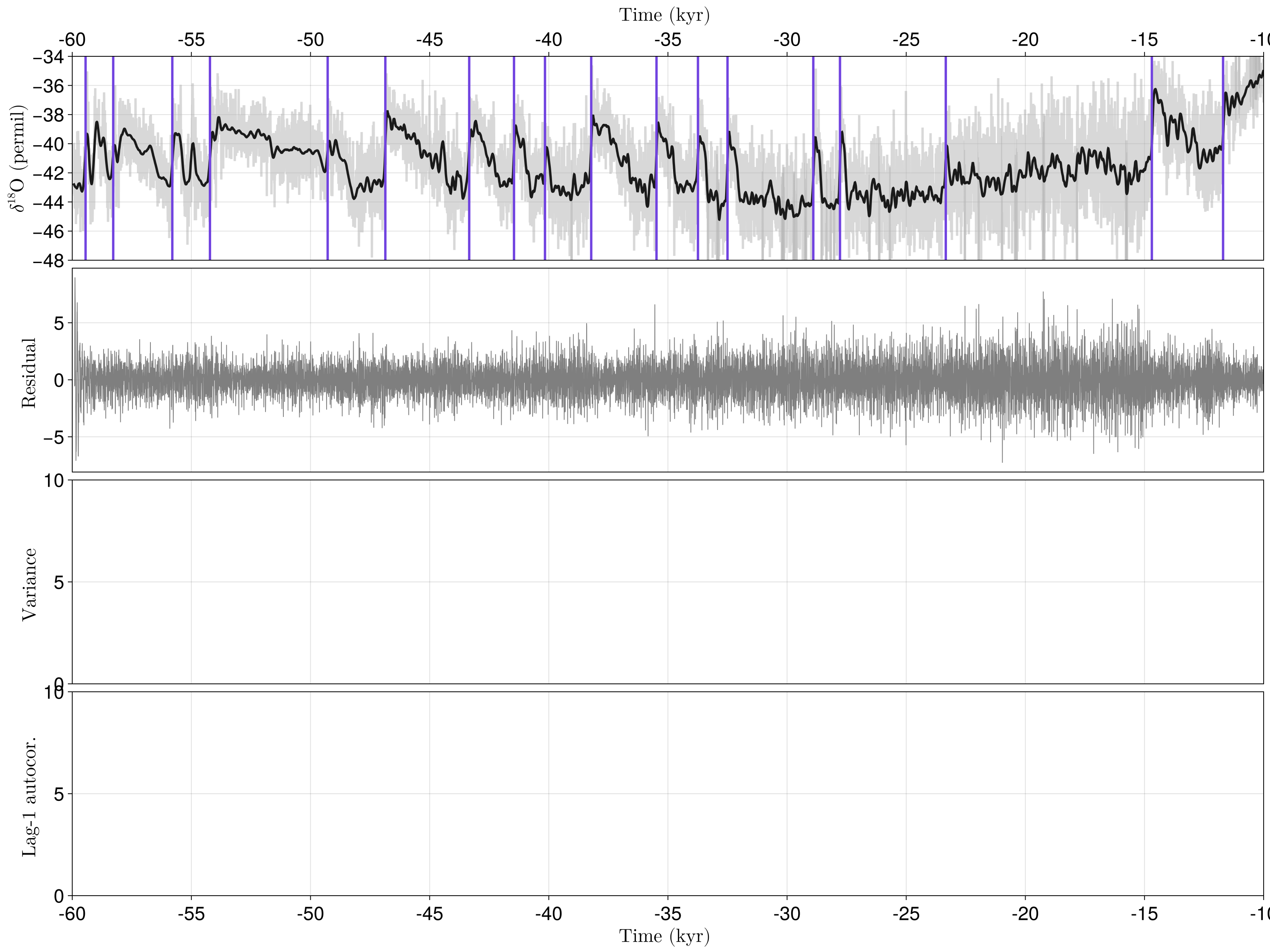

Hindcast on NGRIP data

As one can see... there is not much to see so far. Residuals are impossible to simply eye-ball and we therefore use TransitionsInTimeseries.jl to study the evolution, measured by the ridge-regression slope of the residual's variance and lag-1 autocorrelation (AC1) over time. In many examples of the literature, including (Boers, 2018), the CSD analysis is performed over segments (sometimes only one) of the timeseries, such that a significance value is obtained for each segment. By using SegmentedWindowConfig, dealing with segments can be easily done in TransitionsInTimeseries.jl and is demonstrated here:

using TransitionsInTimeseries, StatsBase
using Random: Xoshiro

ac1(x) = sum(autocor(x, [1]))   # AC1 from StatsBase
indicators = (var, ac1)
change_metrics = (RidgeRegressionSlope(), RidgeRegressionSlope())
tseg_start = t_rasmussen[1:end-1] .+ 200
tseg_end = t_rasmussen[2:end] .- 200
config = SegmentedWindowConfig(indicators, change_metrics,
    tseg_start, tseg_end; whichtime = last, width_ind = Int(200÷dt),
    min_width_cha = 100)        # require >=100 data points to estimate change metric
results = estimate_changes(config, r, t)
signif = SurrogatesSignificance(n = 1000, tail = [:right, :right], rng = Xoshiro(1995))
flags = significant_transitions(results, signif)

18×2 BitMatrix:
 0  0
 0  0
 0  0
 0  0
 1  0
 1  1
 1  1
 1  1
 0  0
 1  0
 1  0
 0  0
 0  0
 1  0
 0  0
 0  0
 1  0
 1  0

That's it! We can now visulaise our results with a generic function that we will re-use later:

function plot_segment_analysis!(axs, results, signif)
    (; t_indicator, x_indicator) = results
    for k in eachindex(t_indicator)             # loop over the segments
        for i in axes(signif.pvalues, 2)        # loop over the indicators
            if !isnan(signif.pvalues[k, i])     # plot if segment long enough
                # Plot indicator timeseries and its linear regression
                ti, xi = t_indicator[k], x_indicator[k][:, i]
                lines!(axs[i+2], ti, xi, color = Cycled(1))
                m, p = ridgematrix(ti, 0.0) * xi
                if signif.pvalues[k, i] < 0.05
                    lines!(axs[i+2], ti, m .* ti .+ p, color = :gray5, linewidth = 3)
                else
                    lines!(axs[i+2], ti, m .* ti .+ p, color = :gray60, linewidth = 3)
                end
            end
        end
    end
end
plot_segment_analysis!(axs, results, signif)
fig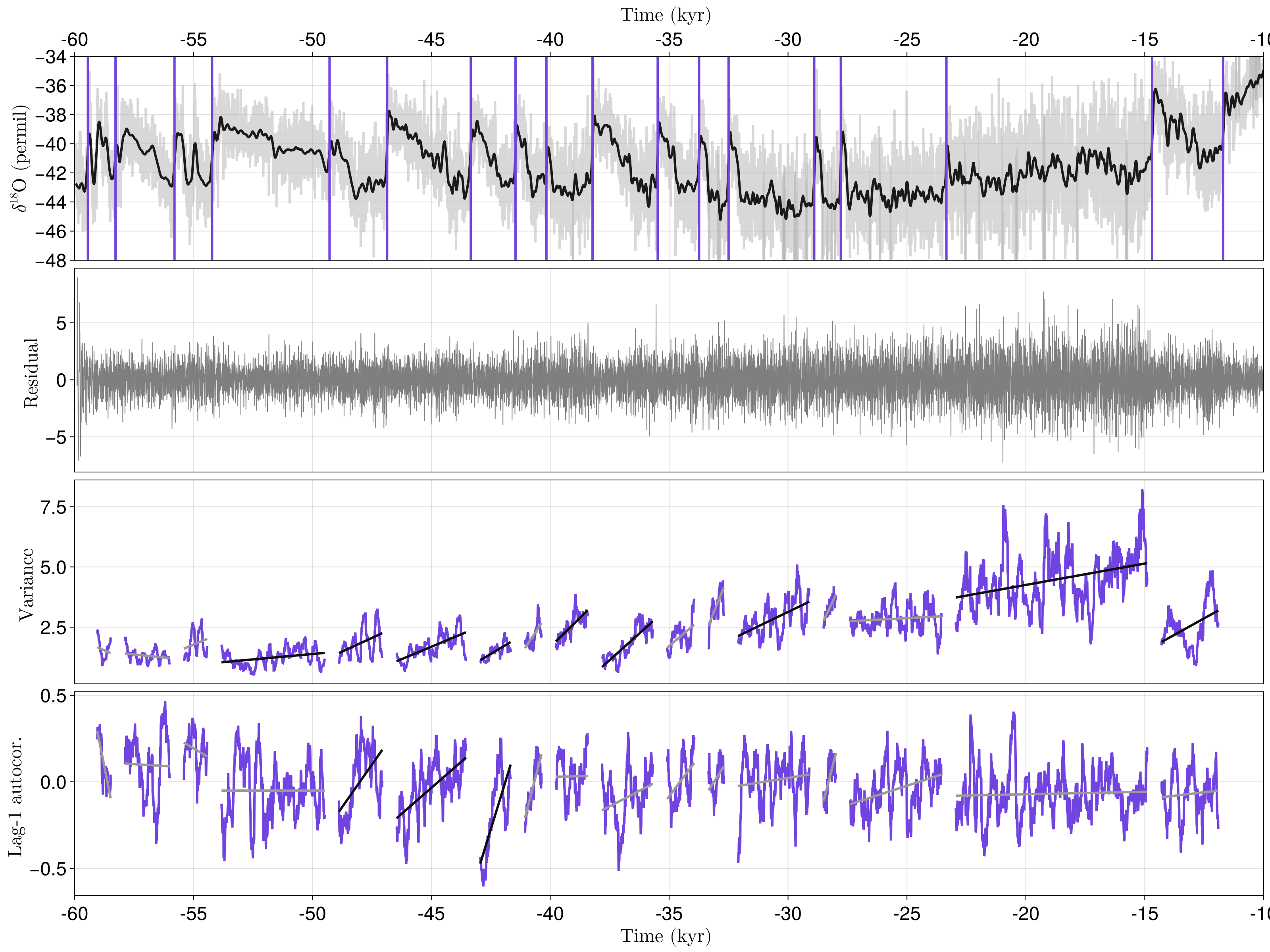

In (Boers, 2018), 13/16 and 7/16 true positives are respectively found for the variance and AC1, with 16 referring to the total number of transitions. The timeseries actually includes 18 transition but, in (Boers, 2018), some segments are considered too small to be analysed. In contrast, we here respectively find 9/16 true positives for the variance and 3/16 for AC1. We can track down the discrepancies to be in the surrogate testing, since the indicator timeseries computed here are almost exactly similar to those of (Boers, 2018). This mismatch points out that packages like TransitionsInTimeseries.jl are wishful for research to be reproducible, especially since CSD is gaining attention - not only within the scientific community but also in popular media.

CSD: only a necessary condition, only in some cases

For codimension-1 systems, approaching a fold, Hopf or transcritical bifurcation implies a widening of the potential $U$, which defines the deterministic term $f = -∇U$ of the SDE's right-hand-side. In the presence of noise, this leads to CSD, which is therefore a necessary condition for crossing one of these bifurcations - although it is not always assessable by analysing the timeseries due to practical limitations (e.g. sparse data subject to large measurement noise). It is nonetheless not given that DO-events, as many other real-life applications, can be seen as a codimension-1 fold, Hopf or transcritical bifurcations. Besides this, we emphasise that CSD is not a sufficient condition for assessing a transition being ahead in near future, since a resilience loss can happen without actually crossing any bifurcation. This can be illustrated on the present example by performing the same analysis only until few hundred years before the transition:

tseg_end = t_rasmussen[2:end] .- 700    # stop analysis 500 years earlier than before
config = SegmentedWindowConfig(indicators, change_metrics,
    tseg_start, tseg_end, whichtime = last, width_ind = Int(200÷dt),
    min_width_cha = 100)
results = estimate_changes(config, r, t)
signif = SurrogatesSignificance(n = 1000, tail = [:right, :right], rng = Xoshiro(1995))
flags = significant_transitions(results, signif)
fig, axs = plot_do(t3, x3, tloess, xloess, t, r, t_rasmussen, xlims, xticks)
plot_segment_analysis!(axs, results, signif)
fig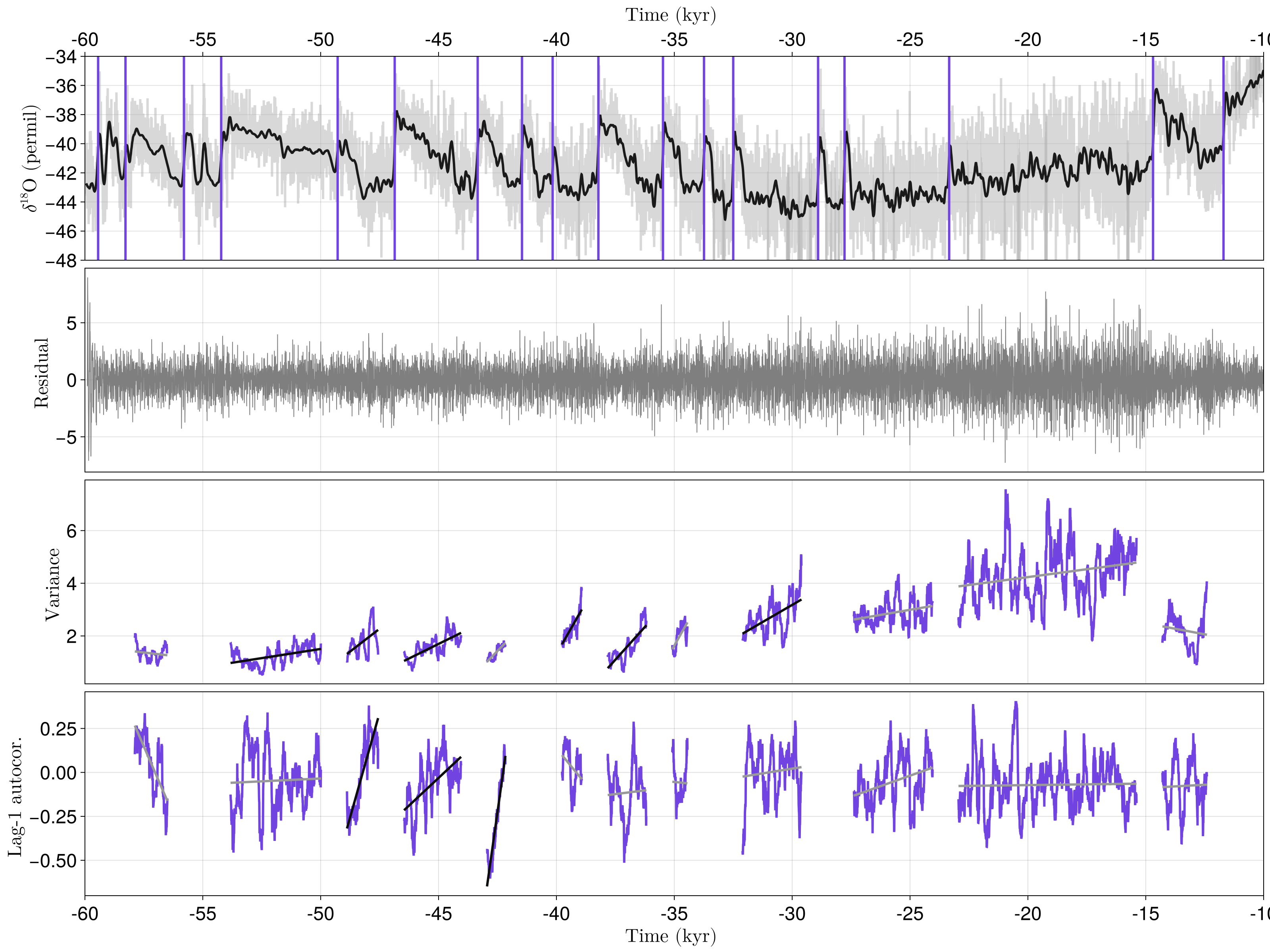

For the variance and AC1, we here respectively find 6 and 3 positives, although the transitions are still far ahead. This shows that what CSD captures is a potential widening induced by a shift of the forcing parameter rather than the actual transition. We therefore believe, as already suggested in some studies, that "resilience-loss indicators" is a more accurate name than "early-warning signals" when using CSD.

We draw attention upon the fact that the $\delta^{18}O$ timeseries is noisy and sparsely re-sampled. Furthermore, interpolating over time introduces a potential bias in the statistics, even if performed on a coarse grid. The NGRIP data therefore represents an example that should be handled with care - as many others where CSD analysis has been applied on transitions in the field of geoscience. To contrast with this, we propose to perform the same analysis on synthethic DO data, obtained from an Earth Model of Intermediate Complexity (EMIC).

Hindcasting simulated DO-events

In CLIMBER-X, the EMIC described in (Willeit et al., 2022), DO-like events can be triggered by forcing the North Atlantic with a (white noise) freshwater input. Simulated DO-like events present the big advantage of being evenly sampled in time and free of measurement noise. We run this analysis over two exemplary simulation outputs:

t_transitions = [[1, 1850, 2970, 3970, 5070, 5810, 7050, 8050],
                 [1, 3500, 4370, 5790, 7200, 8140]]
t_lb = [[300, 500, 300, 600, 300, 500, 500], [1800, 500, 1000, 900, 500]]
tseg_start = [t_transitions[1][1:end-1] + t_lb[1], t_transitions[2][1:end-1] + t_lb[2]]
tseg_end = [t_transitions[1][2:end] .- 50, t_transitions[2][2:end] .- 50]

figvec = Figure[]

for j in 1:2
    # Download the data and perform loess filtering on it
    tmp = Base.download("https://raw.githubusercontent.com/JuliaDynamics/JuliaDynamics/" *
        "master/timeseries/climberx-do$(j)-omaxa.csv")
    data = readdlm(tmp)
    tcx, xcx = data[1, 1000:end], data[2, 1000:end]
    t, x, xtrend, r = loess_filter(tcx, xcx, span = 0.02)

    # Initialize figure
    xlims = (0, last(tcx))
    xticks = kyr_xticks(xlims[1]:1e3:xlims[2])
    fig, axs = plot_do(tcx, xcx,  t, xtrend, t, r, t_transitions[j], extrema(t), xticks)
    ylims!(axs[1], (5, 40))
    axs[1].ylabel = L"Max. Atlantic overturning (Sv) $\,$"

    # Run sliding analysis and update figure with results
    dt = mean(diff(tcx))
    config = SegmentedWindowConfig(
        indicators, change_metrics, tseg_start[j], tseg_end[j],
        whichtime = last, width_ind = Int(200÷dt), min_width_cha = 100)
    results = estimate_changes(config, r, t)
    signif = SurrogatesSignificance(n = 1_000, tail = [:right, :right], rng = Xoshiro(1995))
    flags = significant_transitions(results, signif)

    plot_segment_analysis!(axs, results, signif)
    vlines!(axs[1], t_transitions[j], color = Cycled(1), linewidth = 3)
    push!(figvec, fig)
end
figvec[1]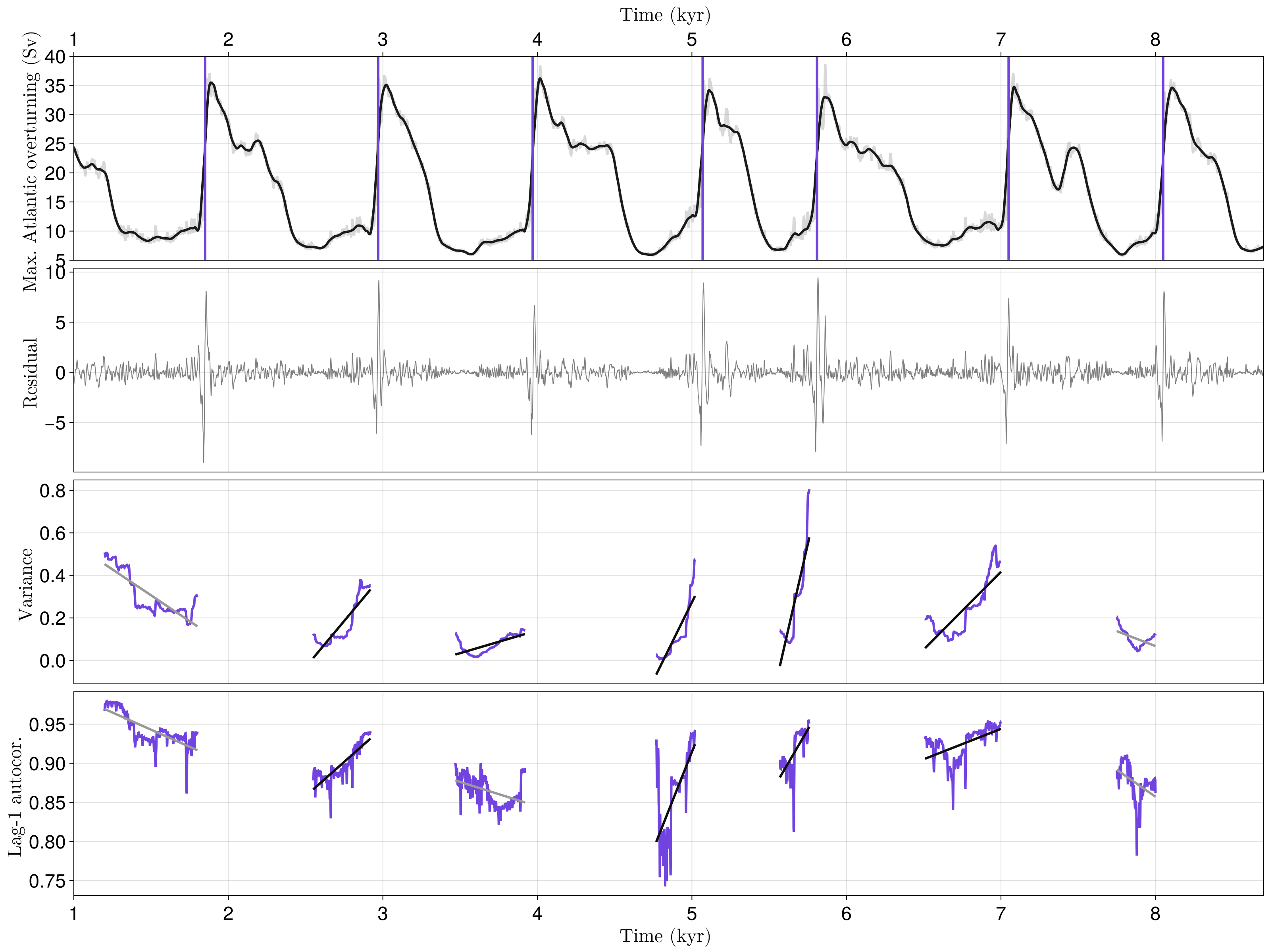

It here appears that not all transitions are preceeded by a significant increase of variance and AC1, even in the case of clean and evenly sampled time series. Let's check another case:

figvec[2]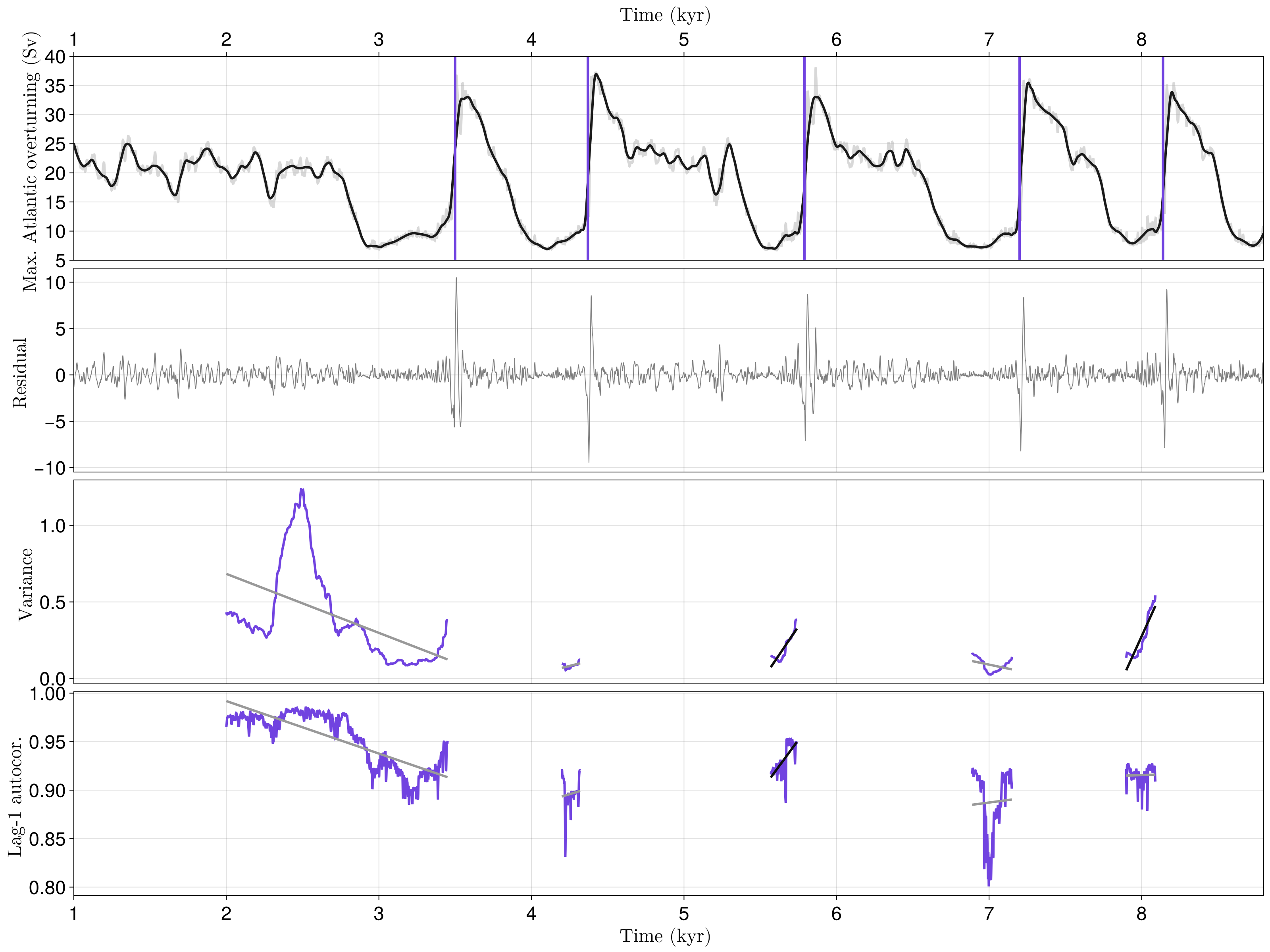

Same here! Although CLIMBER-X does not represent real DO-events, the above-performed analysis might be hinting at the fact that not all DO transitions can be forecasted with CSD. Nonetheless, performing a CSD analysis can inform on the evolution of a system's resilience.