Tutorial

Workflow

Computing transition indicators consists of the following steps:

1. Doing any preprocessing of raw data first, such as detrending. This not part of TransitionsInTimeseries.jl and yields the input timeseries.
2. Estimating the timeseries of an indicator by sliding a window over the input timeseries.
3. Computing the changes of the indicator by sliding a window over its timeseries. Alternatively, the change metric can be estimated over the whole segment, as examplified in the section Segmented windows.
4. Generating many surrogates that preserve important statistical properties of the original timeseries.
5. Performing step 2 and 3 for the surrogate timeseries.
6. Checking whether the indicator change timeseries of the real timeseries shows a significant feature (trend, jump or anything else) when compared to the surrogate data.

These steps are illustrated one by one in the tutorial below, and then summarized in the convenient API that TransitionsInTimeseries.jl exports.

Tutorial – Educational

Raw input data

Let us load data from a bistable nonlinear model subject to noise and to a gradual change of the forcing that leads to a transition. Furthermore, we also load data from a linear model, which is by definition monostable and therefore incapable of transitioning. This is done to control the rate of false positives, a common problem that can emerge when looking for transition indicators. The models are governed by:

\[\dfrac{\mathrm{d}x_{l}}{\mathrm{d}t} = - x_{l} - 1 + f(t) + n(t) \\ \dfrac{\mathrm{d}x_{nl}}{\mathrm{d}t} = - x_{nl}^3 + x_{nl} + f(t) + n(t)\]

with $x_{l}$ the state of the linear model, $x_{nl}$ the state of the bistable model, $f$ the forcing and $n$ the noise. For $f=0$ they both display an equilibrium point at $x=-1$. However, the bistable model also displays a further equilibrium point at $x=1$. Loading (and visualizing with Makie) such prototypical data to test some indicators can be done by simply running:

using TransitionsInTimeseries, CairoMakie

t, x_linear, x_nlinear = load_linear_vs_doublewell()
fig, ax = lines(t, x_linear)
lines!(ax, t, x_nlinear)
ax.title = "raw data"
fig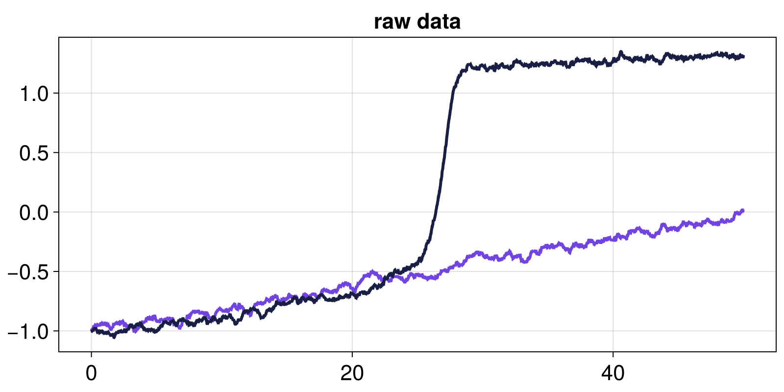

Preprocessing

The nonlinear system clearly displays a transition between two stability regimes. To forecast such transition, we analyze the fluctuations of the timeseries around the attractor, assumed to be tracked. Therefore, a detrending step is needed - here simply obtained by building the difference of the timeseries with lag 1.

x_l_fluct = diff(x_linear)
x_nl_fluct = diff(x_nlinear)
tfluct = t[2:end]

fig, ax = lines(tfluct, x_l_fluct)
lines!(ax, tfluct, x_nl_fluct .+ 0.05)
ax.title = "input timeseries"
fig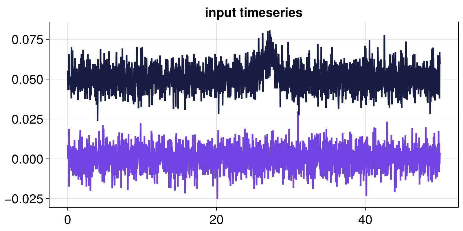

At this point, x_l_fluct and x_nl_fluct are considered the input timeseries.

Indicator timeseries

We can then compute the values of some "indicator" (a Julia function that inputs a timeseries and outputs a number). An indicator should be a quantity that is likely to change if a transition occurs, or is about to occur in the timeseries. We compute indicators by applying a sliding window over the input timeseries, determined by the width and the stride with which it is applied. Here we demonstrate this computation with the AR1-regression coefficient (under white-noise assumption), implemented as ar1_whitenoise:

indicator = ar1_whitenoise
indicator_window = (width = 400, stride = 1)

# By mapping `last::Function` over a windowviewer of the time vector,
# we obtain the last time step of each window.
# This therefore only uses information from `k-width+1` to `k` at time step `k`.
# Alternatives: `first::Function`, `midpoint:::Function`.
t_indicator = windowmap(last, tfluct; indicator_window...)
indicator_l = windowmap(indicator, x_l_fluct; indicator_window...)
indicator_nl = windowmap(indicator, x_nl_fluct; indicator_window...)

fig, ax = lines(t_indicator, indicator_l)
lines!(ax, t_indicator, indicator_nl)
ax.title = "indicator timeseries"
fig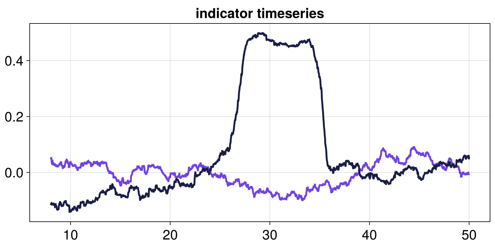

The lines plotted above are the indicator timeseries.

Change metric timeseries

From here, we process the indicator timeseries to quantify changes in it. This step is in essence the same as before: we apply some function over a sliding window of the indicator timeseries. We call this new timeseries the change metric timeseries. In the example here, the change metric we will employ will be the slope (over a sliding window), calculated via means of a RidgeRegressionSlope:

change_window = (width = 30, stride = 1)
ridgereg = RidgeRegressionSlope(lambda = 0.0)
precompridgereg = precompute(ridgereg, t[1:change_window.width])

t_change = windowmap(last, t_indicator; change_window...)
change_l = windowmap(precompridgereg, indicator_l; change_window...)
change_nl = windowmap(precompridgereg, indicator_nl; change_window...)

fig, ax = lines(t_change, change_l)
lines!(ax, t_change, change_nl)
ax.title = "change metric timeseries"
fig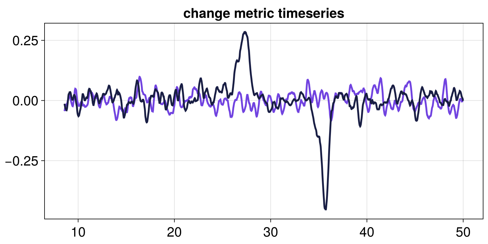

Timeseries surrogates

As expected from Critical Slowing Down, an increase of the AR1-regression coefficient can be observed. Although eyeballing the timeseries might already be suggestive, we want a rigorous framework for testing for significance.

In TransitionsIdentifiers.jl we perform significance testing using the method of timeseries surrogates and the TimeseriesSurrogates.jl Julia package. This has the added benefits of reproducibility, automation and flexibility in choosing the surrogate generation method. Note that TimeseriesSurrogates is re-exported by TransitionsInTimeseries, so that you don't have to using both of them.

To illustrate the surrogate, we compare the change metric computed from the bistable timeseries what that computed from a surrogate of the same timeseries.

# Generate Fourier random-phase surrogates
using Random: Xoshiro
s = surrogate(x_nl_fluct, RandomFourier(), Xoshiro(123))

function gridfig(nrows, ncols)
    fig = Figure()
    axs = [Axis(fig[i, j], xticklabelsvisible = i == nrows ? true : false)
        for j in 1:ncols, i in 1:nrows]
    rowgap!(fig.layout, 10)
    return fig, axs
end
fig, axs = gridfig(2, 1)
lines!(axs[1], tfluct, x_nl_fluct, color = Cycled(2))
lines!(axs[1], tfluct, s .- 0.05, color = Cycled(3))
axs[1].title = "real signal vs. surrogate(s)"

# compute and plot indicator and change metric
indicator_s = windowmap(indicator, s; indicator_window...)
change_s = windowmap(precompridgereg, indicator_s; change_window...)

lines!(axs[2], t_change, change_nl, label = "nonlin", color = Cycled(2))
lines!(axs[2], t_change, change_s, label = "surrogate", color = Cycled(3))
axislegend()
axs[2].title = "change metric"

[xlims!(ax, 0, 50) for ax in axs]
fig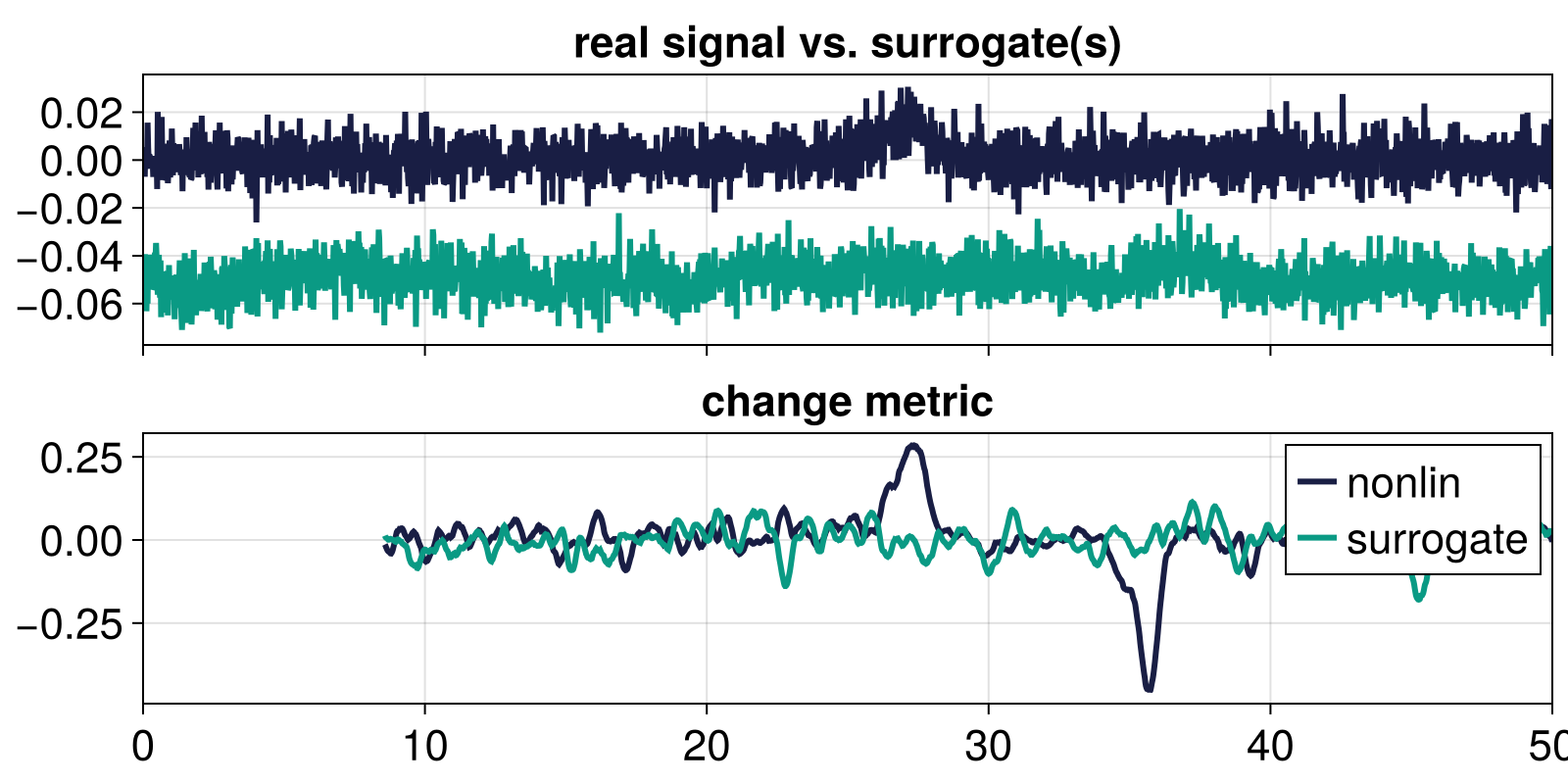

Quantifying significance

To quantify the significance of the values of the change metric timeseries we perform a standard surrogate test by computing the p-value w.r.t. the change metrics of thousands of surrogates of the input timeseries. A low p-value (typically p<0.05) is commonly considered as significant. To visualize significant trends, we plot the p-value vs. time:

n_surrogates = 1_000
fig, axs = gridfig(2, 2)
axs[1].title = "linear"
axs[2].title = "nonlinear"

for (j, ax, axsig, x) in zip(1:2, axs[1:2], axs[3:4], (x_l_fluct, x_nl_fluct))

    orig_change = j == 1 ? change_l : change_nl
    sgen = surrogenerator(x, RandomFourier(), Xoshiro(123))
    pval = zeros(length(change_s))

    # Collect all surrogate change metrics
    for i in 1:n_surrogates
        s = sgen()
        indicator_s = windowmap(indicator, s; indicator_window...)
        change_s = windowmap(precompridgereg, indicator_s; change_window...)
        pval += orig_change .< change_s
    end

    pval ./= n_surrogates
    lines!(ax, t_change, orig_change)   # ; color = Cycled(j)
    lines!(axsig, t_change, pval)       # ; color = Cycled(j+2)
end

[xlims!(ax, 0, 50) for ax in axs]
fig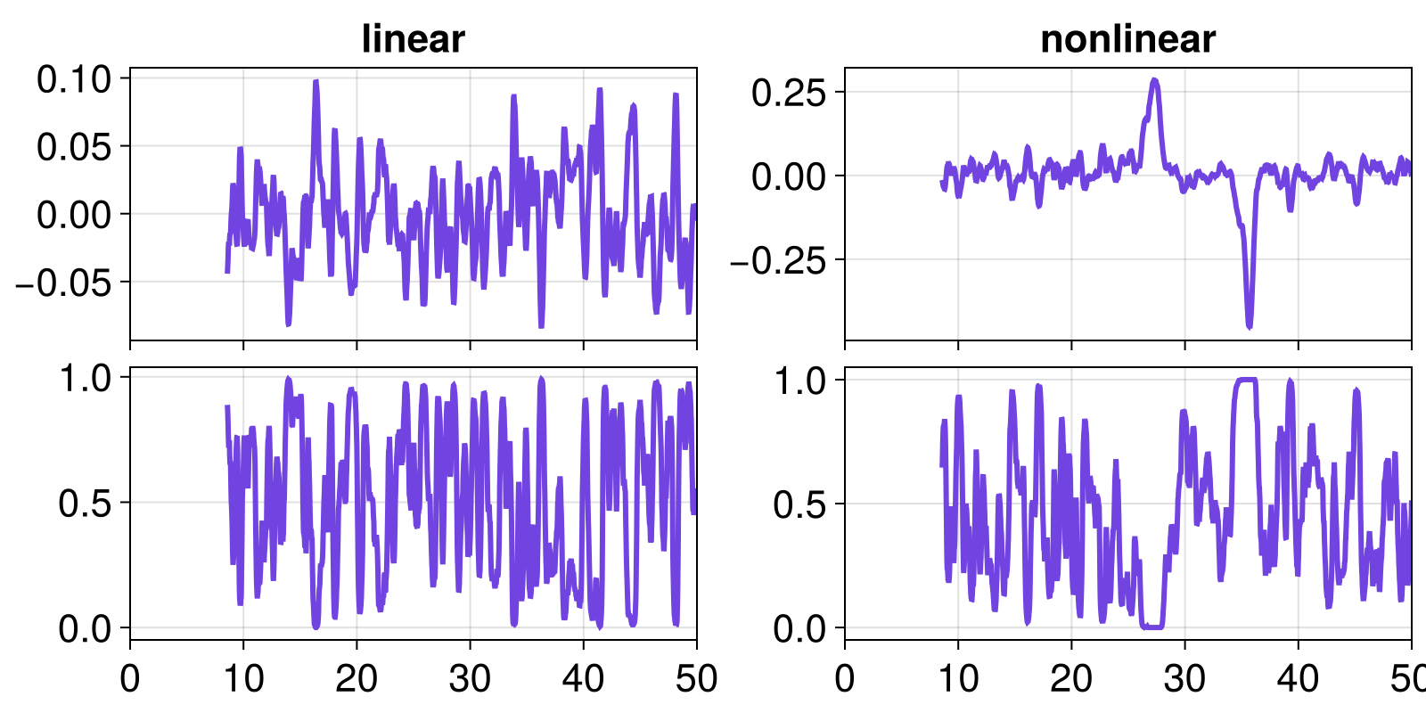

As expected, the data generated by the nonlinear model displays a significant increase of the AR1-regression coefficient before the transition, which is manifested by a low p-value. In contrast, the data generated by the linear model does not show anything similar.

Performing the step-by-step analysis of transition indicators is possible and might be preferred for users wanting high flexibility. However, this results in a substantial amount of code. We therefore provide convenience functions that wrap this analysis, as shown in the next section.

Tutorial – TransitionsInTimeseries.jl

TransitionsInTimeseries.jl wraps this typical workflow into a simple, extendable, and modular API that researchers can use with little effort. In addition, it allows performing the same analysis for several indicators / change metrics in one go.

The interface is simple, and directly parallelizes the Workflow. It is based on the creation of a ChangesConfig, which contains a list of indicators, and corresponding metrics, to use for doing the above analysis. It also specifies what kind of surrogates to generate.

Sliding windows

The following blocks illustrate how the above extensive example is re-created in TransitionsInTimeseries.jl

using TransitionsInTimeseries, CairoMakie

t, x_linear, x_nlinear = load_linear_vs_doublewell()

# input timeseries and time
input = x_nl_fluct = diff(x_nlinear)
t = t[2:end]

fig, ax = lines(t, input)
ax.title = "input timeseries"
fig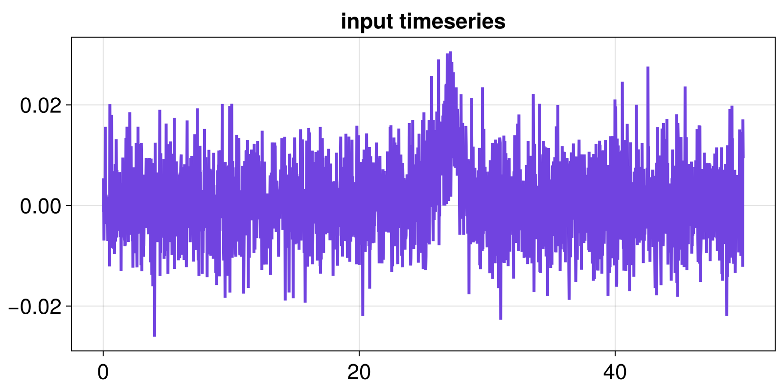

To perform all of the above analysis we follow a 2-step process.

Step 1, we decide what indicators and change metrics to use in SlidingWindowConfig and apply those via a sliding window to the input timeseries using estimate_changes.

# These indicators are suitable for Critical Slowing Down
indicators = (var, ar1_whitenoise)

# use the ridge regression slope for both indicators
change_metrics = (RidgeRegressionSlope(), RidgeRegressionSlope())

# choices go into a configuration struct
config = SlidingWindowConfig(indicators, change_metrics;
    width_ind = 400, width_cha = 30, whichtime = last)

# choices are processed
results = estimate_changes(config, input, t)

SlidingWindowResults
 input timeseries:              2500-element Vector{Float64}
 indicators:                    [:var, :ar1_whitenoise]
 indicator (window, stride):    (400, 1)
 change metrics:                [:PrecomputedRidgeRegressionSlope, :PrecomputedRidgeRegressionSlope]
 change metric (window, stride): (30, 1)

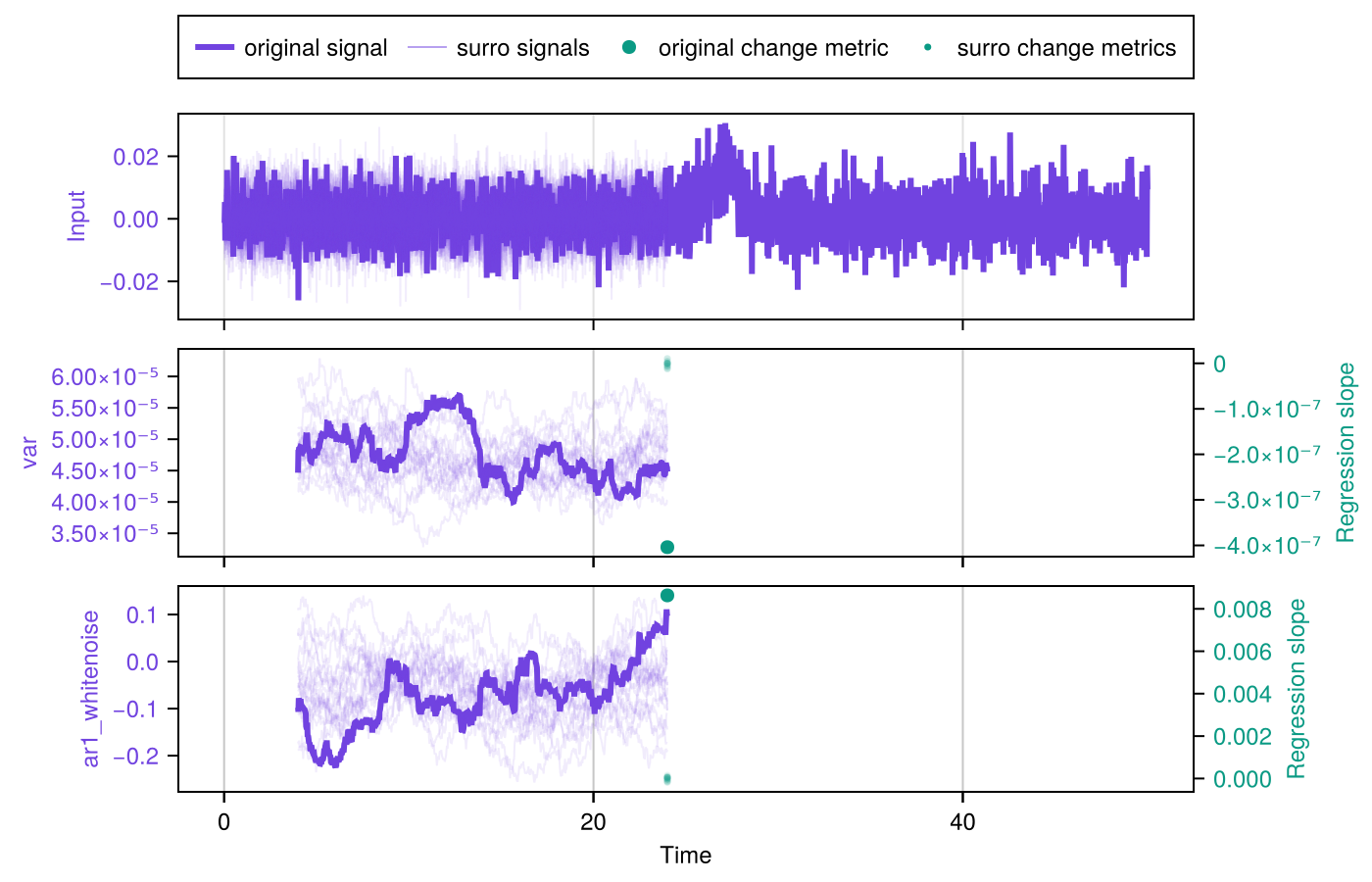
We can conveniently plot the information contained in results by using plot_indicator_changes:

fig = plot_indicator_changes(results)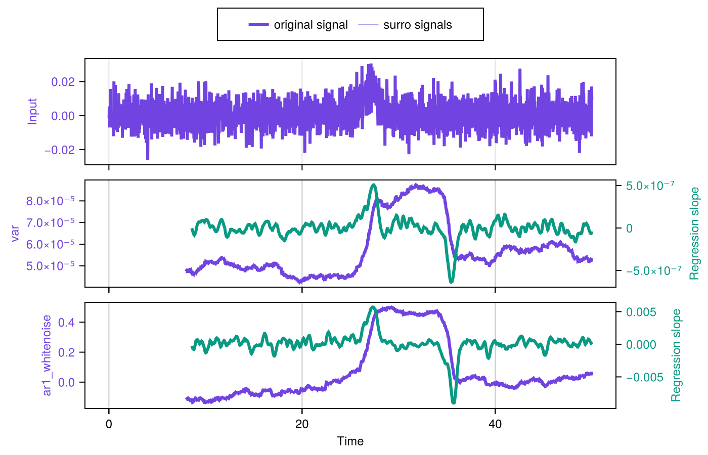

Step 2 is to estimate significance using SurrogatesSignificance and the function significant_transitions. Finally, we can conveniently plot the results obtained by updating the figure obtained above with plot_significance!:

signif = SurrogatesSignificance(n = 1000, tail = [:right, :right])
flags = significant_transitions(results, signif)
plot_significance!(fig, results, signif, flags = flags)
fig

Segmented windows

The analysis shown so far relies on sliding windows of the change metric. This is particularly convenient for transition detection tasks. Segmented windows for the change metric computation are however preferable when it comes to prediction tasks. By only slightly modifying the syntax used so far, one can perform the same computations on segmented windows, as well as visualise the results conveniently:

config = SegmentedWindowConfig(indicators, change_metrics,
    t[1:1], t[1200:1200]; whichtime = last, width_ind = 200,
    min_width_cha = 100)
results = estimate_changes(config, input, t)
signif = SurrogatesSignificance(n = 1000, tail = [:right, :right])
flags = significant_transitions(results, signif)
fig = plot_changes_significance(results, signif)