Kolmogorov-Smirnov test for detecting transitions in paleoclimate timeseries

The goal of this example is to show how simple it is to re-create an analysis similar to what was done in the paper "Automatic detection of abrupt transitions in paleoclimate records", (Bagniewski et al., 2021). The same analysis was then used to create a database of transitions in paleoclimate records in (Bagniewski et al., 2023) Using TransitionsInTimeseries.jl and HypothesisTests.jl, the analysis becomes a 10-lines-of-code script (for a given timeseries).

Scientific background

The approach of (Bagniewski et al., 2021) is based on the two-sample Kolmogorov Smirnov test. It tests whether the samples from two datasets or timeseries are distributed according to the same cumulative density function or not. This can be estimated by comparing the value of the KS-statistic versus some threshold that depends on the required confidence.

The application of this test for identifying transitions in timeseries is simple:

1. A sliding window analysis is performed in the timesries
2. In each window, the KS statistic is estimated between the first half and the second half of the timeseries within this window.
3. Transitions are defined by when the KS statistic exceeds a particular value based on some confidence. The transition occurs in the middle of the window.

We should point out that in (Bagniewski et al., 2021) the authors did a more detailed analysis: analyzed many different window widths, added a conditional clause to exclude transitions that do not exceed a predefined minimum "jump" in the data, and also added another conditional clause that filtered out transitions that are grouped in time (which is a natural consequence of using the Kolmogorov-Smirov test for detecting transitions).

Here we won't do that post processing, mainly because it is rather simple to include these additional conditional clauses to filter transitions after they are found.

Steps for TransitionsInTimeseries.jl

Doing this kind of work with TransitionsInTimeseries.jl is so easy you won't even trip! This analysis follows the same sliding window approach showcased in our Tutorial, and it even excludes the "indicator" aspect: the change metric is estimated directly from the input data!

As such, we really only need to define/do these things before we have finished the analysis:

1. Load the input data (we will use the same example as the NGRIP data of Dansgaard-Oescher events and Critical Slowing Down example) and set the appropriate time window.
2. Define the function that estimates the change metric (i.e., the KS-statistic)
3. Perform the sliding window analysis as in the Tutorial with estimate_changes
4. Estimate the "confident" transitions in the data by comparing the estimated KS-statistic with a predefined threshold.

Load timeseries and window length

Following the Dansgaard-Oescher events example, we load the data after all the processing steps done in that example:

using DelimitedFiles, CairoMakie

tmp = Base.download("https://raw.githubusercontent.com/JuliaDynamics/JuliaDynamics/"*
    "master/timeseries/NGRIP_processed.csv")
data = readdlm(tmp)
t, xtrend, xresid, xloess = collect.(eachcol(data))

fig, ax = lines(t, xtrend; axis = (ylabel = "NGRIP (processed)", xlabel = "time"))
lines!(ax, t, xloess; linewidth = 2)
fig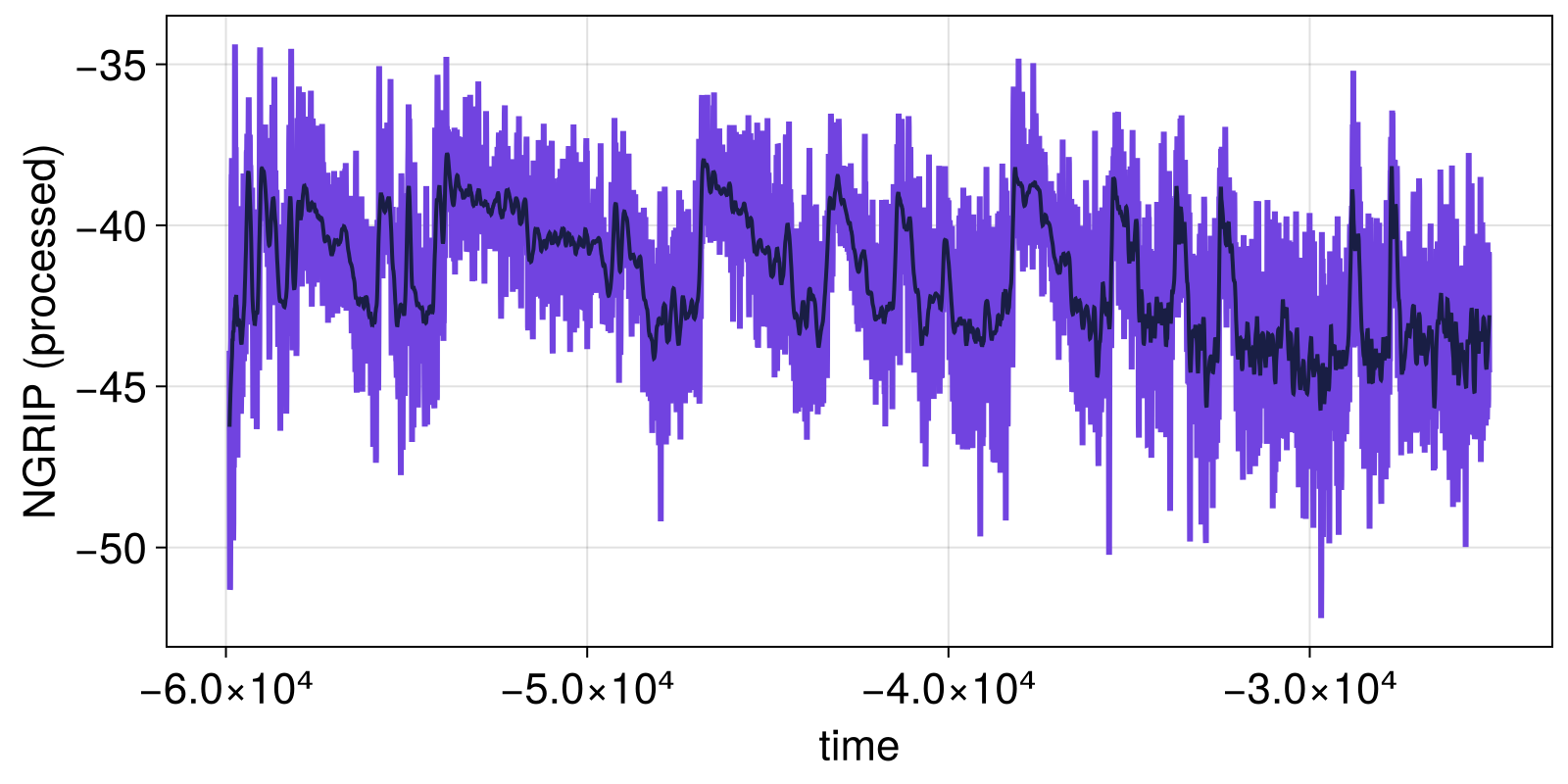

For the window, since we are using a sliding window here, we will be using a window of length 500 (which is approximately 1/2 to 1/4 the span between typical transitions found by (Rasmussen et al., 2014)).

window = 500

500

Defining the change metric function

HypothesisTest.jl implements the Kolmogorov-Smirnov test, however here we are interested in the value of the test iself (the so-called KS-statistic), rather than a p-value. To this end, we define the following function to compute the statistic, which also normalizes it as in (Bagniewski et al., 2021).

using HypothesisTests

function normalized_KS_statistic(timeseries)
    N = length(timeseries)
    i = N÷2
    x = view(timeseries, 1:i)
    y = view(timeseries, (i+1):N)
    kstest = ApproximateTwoSampleKSTest(x, y)
    nx = ny = i # length of each timeseries half of total
    n = nx*ny/(nx + ny) # written fully for concreteness
    D_KS = kstest.δ # can be compared directly with sqrt(-log(α/2)/2)
    # Rescale according to eq. (5) of the paper
    rescaled = 1 - ((1 - D_KS)/(1 - sqrt(1/n)))
    return rescaled
end

N = 1000 # the statistic is independent of `N` for large enough `N`!
x = randn(N)
y = 1.8randn(N) .+ 1.0
z = randn(N)
w = 0.6randn(N) .- 2.0

fig, ax = density(x; color = ("black", 0.5), strokewidth = 4.0, label = "reference distribution")
ax.title = "showcase of normalized KS-statistic"
for q in (y, z, w)
    D_KS = normalized_KS_statistic(vcat(x, q))
    density!(ax, q; label = "D_KS = $(D_KS)")
end
axislegend(ax)
fig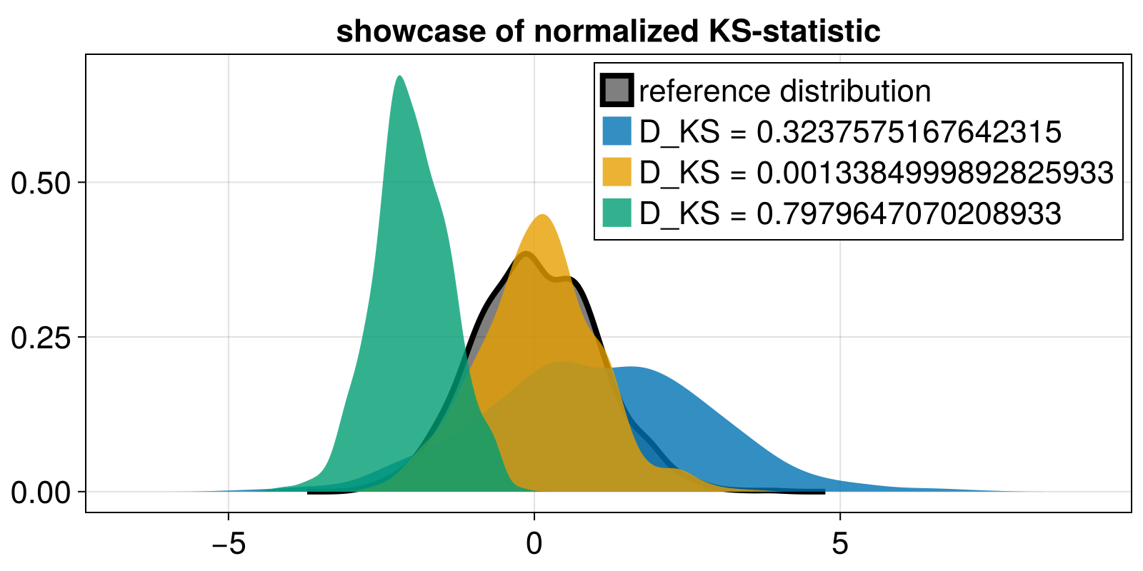

Perform the sliding window analysis

This is just a straightforward call to estimate_changes. In fact, it is even simpler than the tutorial. Here we skip completely the "indicator" estimation step, and we evaluate the change metric directly on input data. We do this by simply passing nothing as the indicators.

using TransitionsInTimeseries

config = SlidingWindowConfig(nothing, normalized_KS_statistic; width_cha = 500)

results = estimate_changes(config, xtrend, t)

SlidingWindowResults
 input timeseries:              6975-element Vector{Float64}
 indicators:                    nothing
 indicator (window, stride):    (100, 1)
 change metrics:                [:normalized_KS_statistic]
 change metric (window, stride): (500, 1)

Which we can visualize

function visualize_results(results)
    fig, ax1 = lines(t, xtrend; axis = (ylabel = "NGRIP (processed)",))
    ax2, = lines(fig[2, 1], results.t_change, vec(results.x_change), axis = (ylabel = "D_KS (normalized)", xlabel = "time"))
    linkxaxes!(ax1, ax2)
    hidexdecorations!(ax1; grid = false)
    xloess_normed = (xloess .- minimum(xloess))./(maximum(xloess) - minimum(xloess))
    lines!(ax2, t, xloess_normed; color = ("gray", 0.5))
    fig
end

visualize_results(results)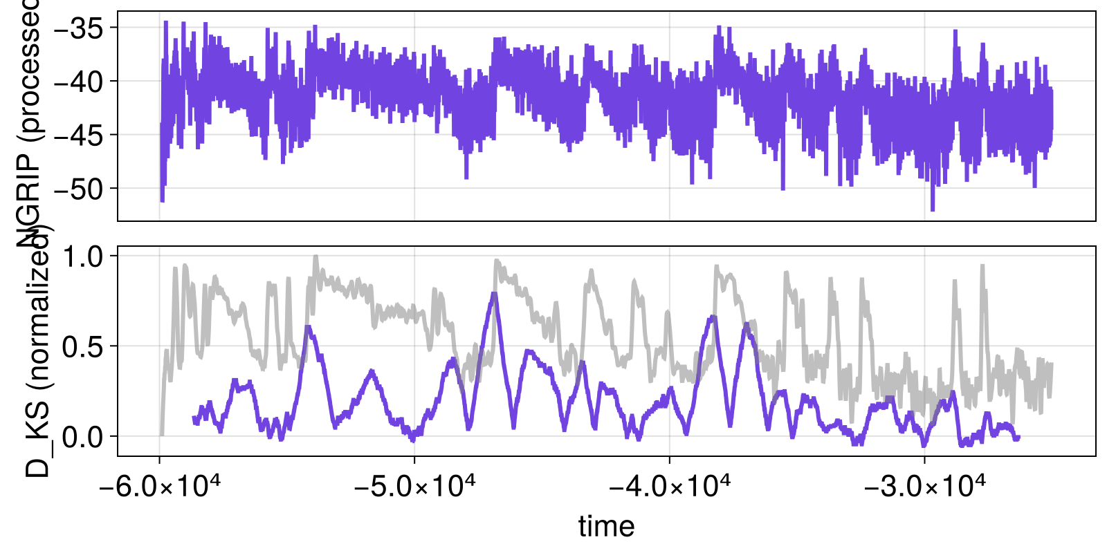

By overplotting the (smoothened) NGRIP timeseries and the normalized KS-statistic, it already becomes pretty clear that the statistic peaks when transitions occur.

The same thing happens if we alter the window duration

config = SlidingWindowConfig(nothing, normalized_KS_statistic; width_cha = 200)
results = estimate_changes(config, xtrend, t)
visualize_results(results)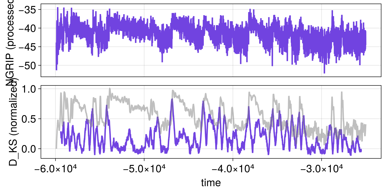

So one can easily obtain extra confidence by varying window size as in (Bagniewski et al., 2021).

Identifying "confident" transitions

As this identification here is done via a simple threshold, identifying the transitions is a nearly trivial call to significant_transitions with ThresholdSignificance

signif = ThresholdSignificance(0.5) # or any other threshold
flags = significant_transitions(results, signif)

fig = visualize_results(results)
axDKS = content(fig[2,1])
vlines!(axDKS, results.t_change[vec(flags)], color = ("red", 0.25))
fig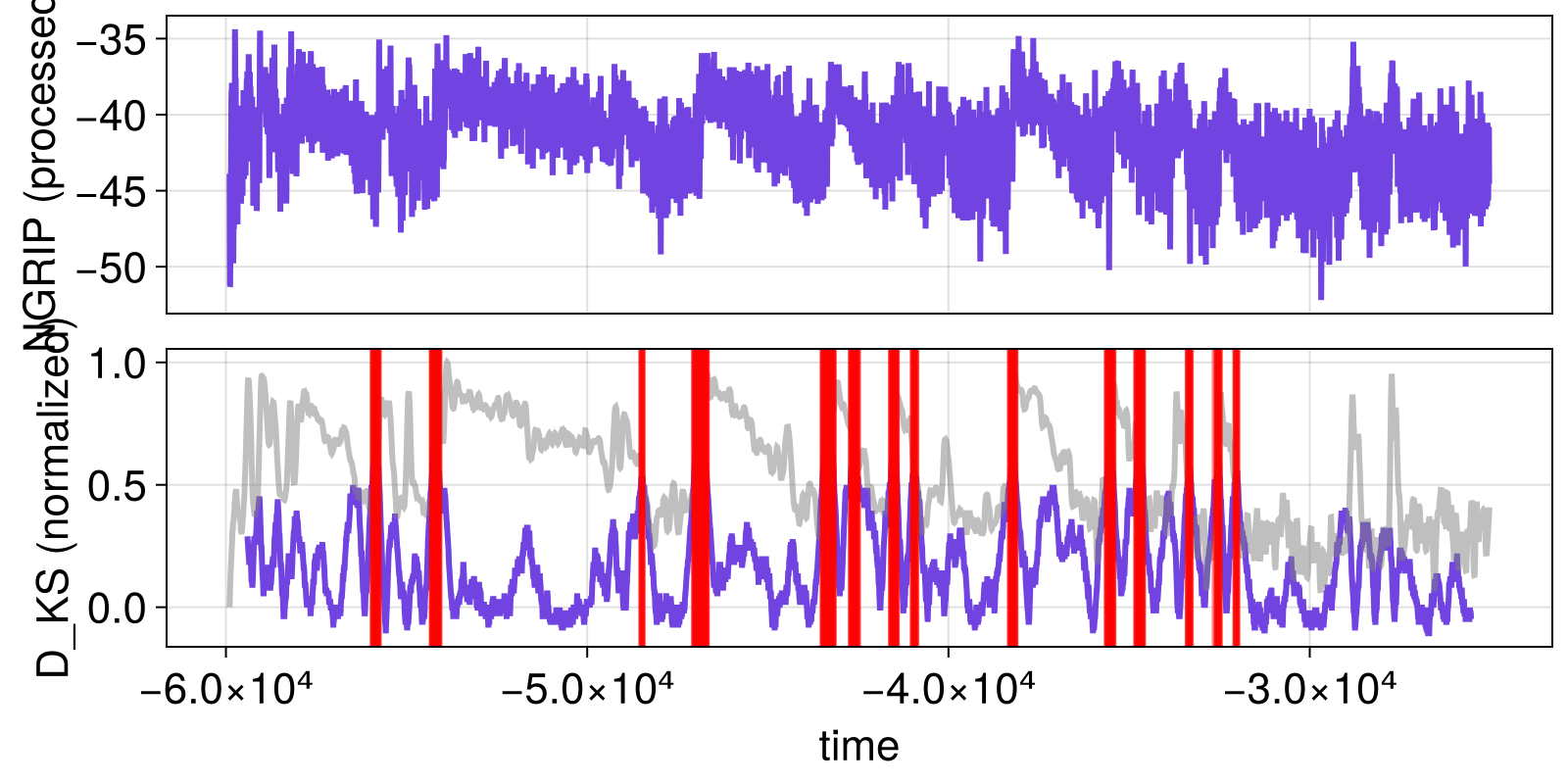

We could proceed with a lot of preprocessing as in (Bagniewski et al., 2021) but we skip this here for the sake of simplicity.