Permutation entropy for dynamic regime changes

Permutation entropy is used frequently to detect a transition between one dynamic regime to another. It is useful when the mean and std. of the timeseries values are very similar between the two regimes, which would mean that common distribution-based indicators, or common critical-slowing-down based indicators, would fail.

This example will also explore different ways to test for significance that are arguably better suitable in such an application than the Tutorial's default of significance via random Fourier surrogates.

Logistic map timeseries

A simple example of this is transitions from periodic to weakly chaotic to chaotic motion in the logistic map. First, let's generate a timeseries of the logistic map

using DynamicalSystemsBase
using CairoMakie

# time-dependent logistic map, so that the `r` parameter increases with time
r1 = 3.83
r2 = 3.86
N = 2000
rs = range(r1, r2; length = N)

function logistic_drifting_rule(u, rs, n)
    r = rs[n+1] # time is `n`, starting from 0
    return SVector(r*u[1]*(1 - u[1]))
end

ds = DeterministicIteratedMap(logistic_drifting_rule, [0.5], rs)
x = trajectory(ds, N-1)[1][:, 1]

2000-element Vector{Float64}:
 0.5
 0.9575
 0.15585767321160574
 0.5039019545917718
 0.9574529422362281
 0.15602441103002537
 0.5043473227583317
 0.9574501255597653
 0.1560361152301728
 0.5043840906474082
 ⋮
 0.4253904015445437
 0.9434836074964187
 0.20581843730311683
 0.6309301050251992
 0.8988117342940414
 0.3510584545931264
 0.8793611090928393
 0.40948549063776396
 0.9333718681550522

Plot it, using as time the parameter value (they coincide)

fig, ax = lines(rs, x; linewidth = 0.5)
ax.xlabel = "r (time)"
ax.ylabel = "x"
fig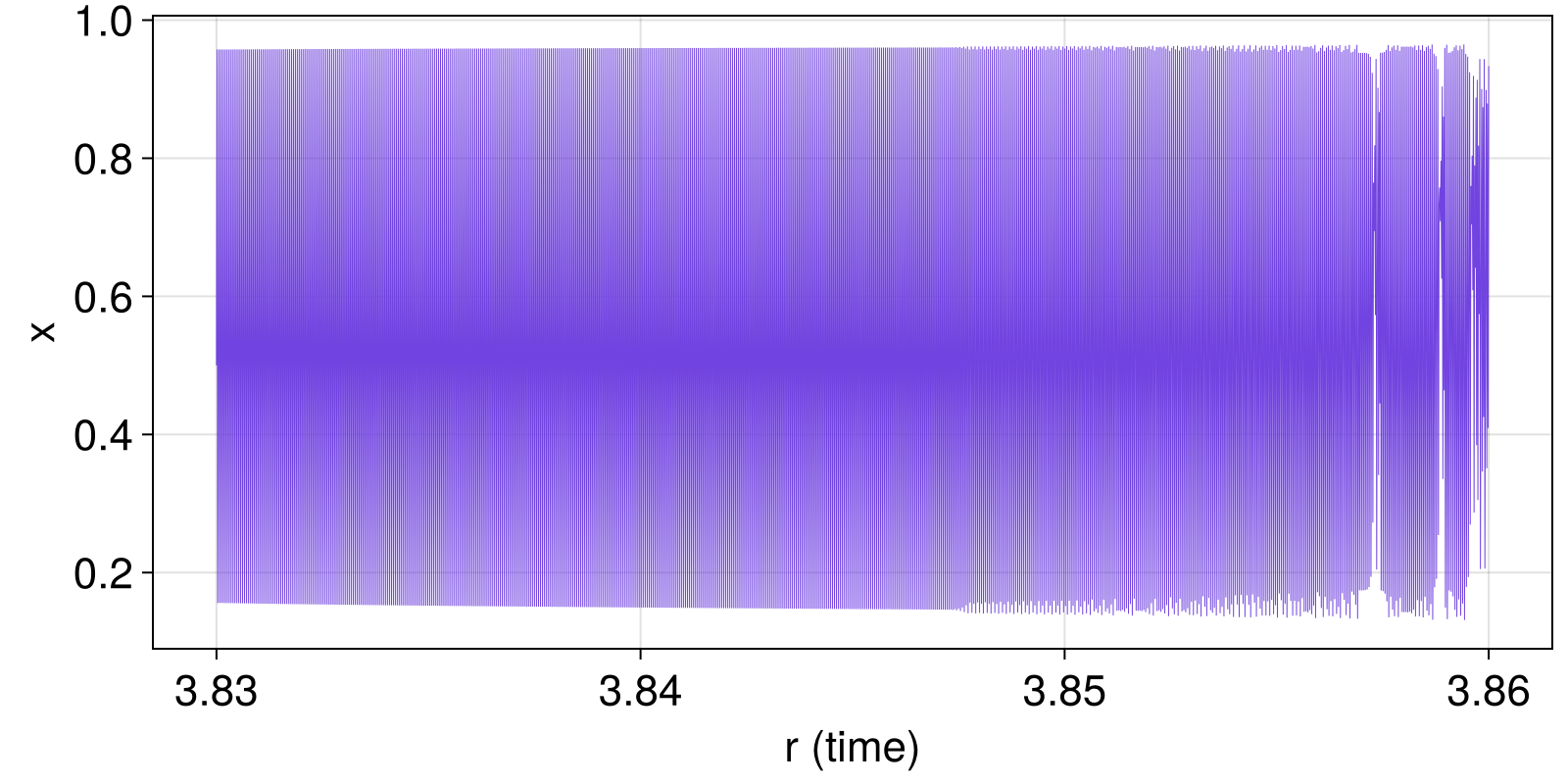

In this example there is a rather obvious transition to strongly chaotic motion at r ≈ 3.855. However, there is also a subtle transition to weak chaos at r ≈ 3.847. This transition is barely visible in the timeseries, and in fact many of the timeseries statistical properties remain identical.

Using a simpler change metric

Now, let's compute and various indicators and their changes, focusing on the permutation entropy as an indicator. We use order 4 here, because we know that to detect changes in a period m we would need an order ≥ m+1 permutation entropy.

using TransitionsInTimeseries, ComplexityMeasures

function permutation_entropy(m)
    est = SymbolicPermutation(; m) # order 3
    indicator = x -> entropy_normalized(est, x)
    return indicator
end

indicators = (var, ar1_whitenoise, permutation_entropy(4))
indistrings = ("var", "ar1", "pe")

("var", "ar1", "pe")

In this example there is no critical slowing down; instead, there is a sharp transition between periodic and chaotic motion. Hence, we shouldn't be using any trend-based change metrics. Instead, we will use the most basic change metric, difference_of_means. With this metric it also makes most sense to use as stride half the window width

metric = (difference_of_means, difference_of_means, difference_of_means)

width_ind = N÷100
width_cha = 20
stride_cha = 10

config = SlidingWindowConfig(indicators, metric;
    width_ind, width_cha, stride_cha,
)

results = estimate_changes(config, x, rs)

SlidingWindowResults
 input timeseries:              2000-element Vector{Float64}
 indicators:                    [:var, :ar1_whitenoise, Symbol("#1")]
 indicator (window, stride):    (20, 1)
 change metrics:                [:difference_of_means, :difference_of_means, :difference_of_means]
 change metric (window, stride): (20, 10)

Let's now plot the change metrics of the indicators

function plot_change_metrics()
    fig, ax = lines(rs, x; axis = (ylabel = "input",), figure = (size = (600, 600),))
    hidexdecorations!(ax; grid = false)
    # plot all change metrics
    for (i, c) in enumerate(eachcol(results.x_change))
        ax, = scatterlines(fig[i+1, 1], results.t_change, c;
            axis = (ylabel = indistrings[i],), label = "input"
        )
        if i < 3
            hidexdecorations!(ax; grid = false)
        else
            ax.xlabel = "r (time)"
        end
    end
    return fig
end

fig = plot_change_metrics()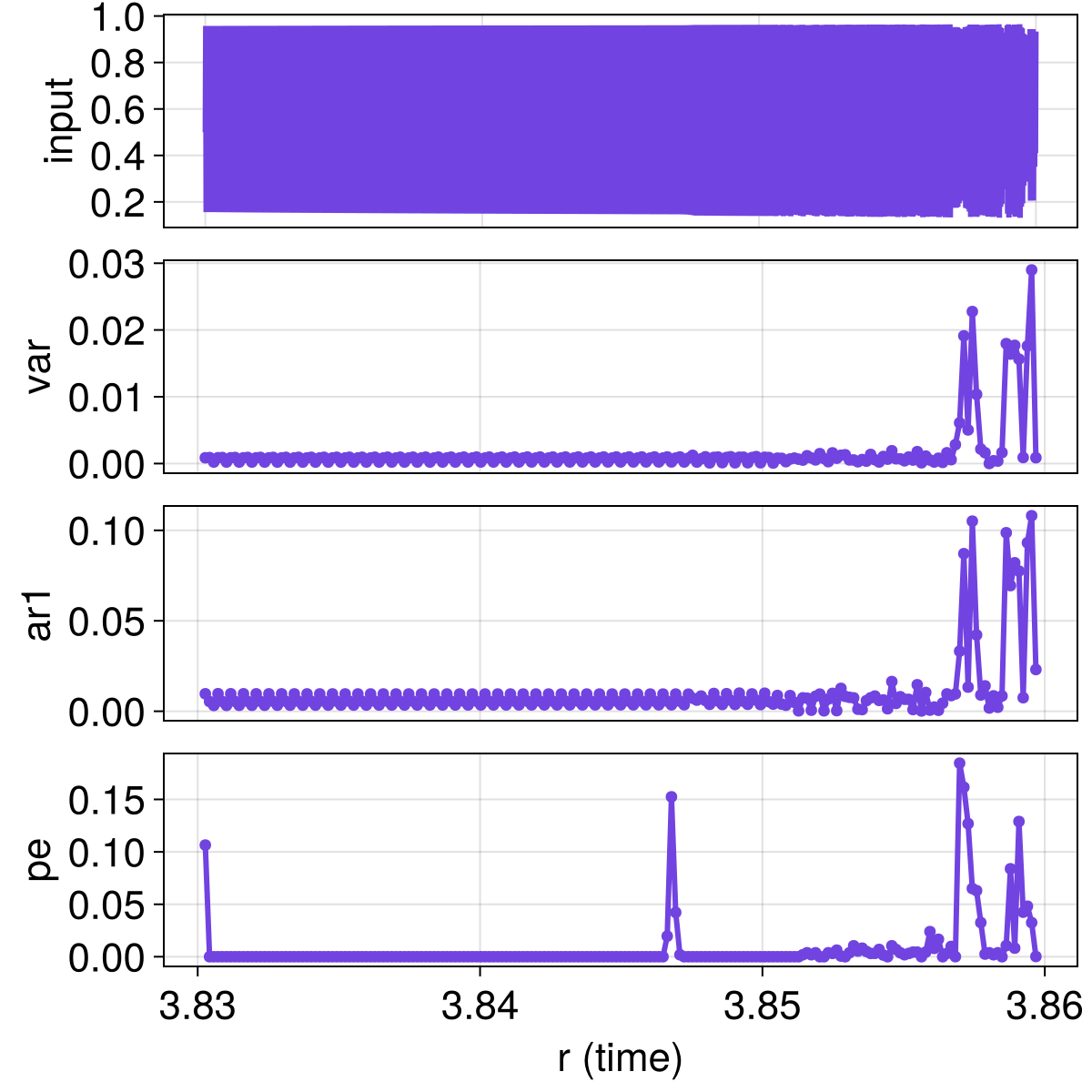

We already see the interesting results we expect: the permutation entropy shows a striking change as we go from periodic to weakly chaotic motion at r ≈ 3.847. (Remember: the plotted quantity is how much the indicator changes within a time window. High values mean large changes.)

Due to its construction, permutation entropy will have a spike for periodic data at the start of the timeseries, so we can safely ignore the spike at r ≈ 3.83.

Significance via random Fourier surrogates

One way to test for significance would be via the standard way as in the Tutorial, utilizing surrogate timeseries and SurrogatesSignificance.

Let's do it here for an example, but, we have to be careful. It is crucial that for permutation entropy we use :right as the tail, because it is expected that the surrogates will have higher differences in the permutation entropy timeseries (because, if there is no dynamical change, the permutation entropy will stay the same, while in the surrogates there are always random fluctuations!

surromethod = RandomFourier()

# Define a function because we will re-use later
using Random: Xoshiro
function overplot_surrogate_significance!(fig, surromethod, color = "black")

    signif = SurrogatesSignificance(;
        n = 1000, tail = [:both, :both, :right], surromethod, rng = Xoshiro(42),
    )
    flags = significant_transitions(results, signif)

    # and also plot the flags with same color
    for (i, indicator) in enumerate(indicators)
        # To make things visually clear, we will also plot some example surrogate
        # timeseries for each indicator and change metric pair
        for _ in 1:10
            s = TimeseriesSurrogates.surrogate(x, surromethod)
            p = windowmap(indicator, s; width = width_ind)
            q = windowmap(metric[i], p; width = width_cha, stride = stride_cha)
            lines!(fig[i+1, 1], results.t_change, q;  color = (color, 0.2), linewidth = 1)
        end
        # Plot the flags as vertical dashed lines
        vlines!(fig[i+1, 1], results.t_change[flags[:, i]];
            color = color, linestyle = :dash, linewidth = 3
        )
    end
    # add a title to the figure with how we estimate significance
    content(fig[1, 1]).title = "surrogates: "*string(nameof(typeof(surromethod)))
end

surromethod = RandomFourier()
overplot_surrogate_significance!(fig, surromethod)

fig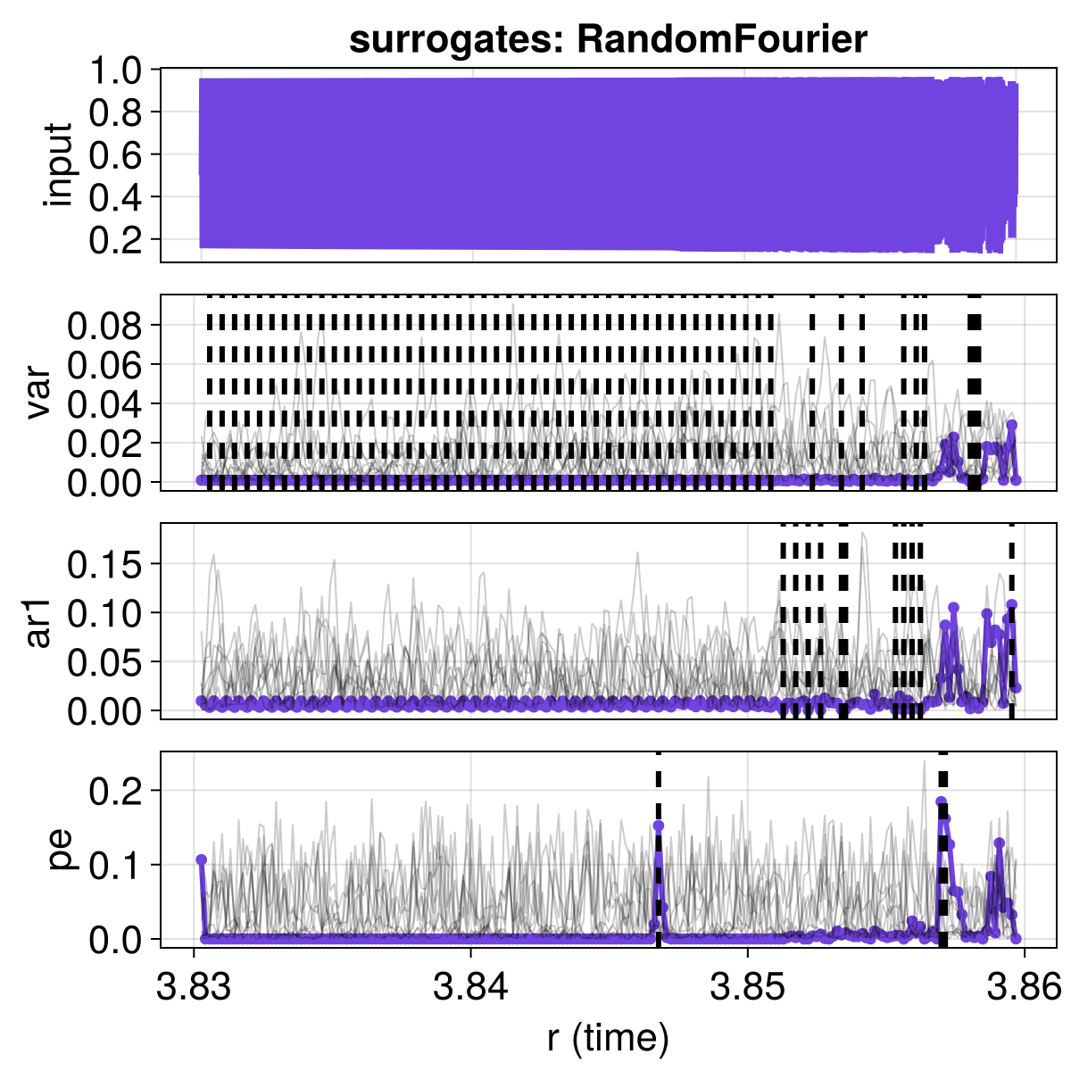

Different surrogates

Random Fourier surrogates perserve the power spectrum of the timeseries, but the power spectrum is a property integrated over the whole timeseries. It doesn't contain any information highlighting the local dynamics or information that preserves the local changes of dynamical behavior.

A surrogate type that does a better job in preserving local sharp changes in the timeseries (and hence provides stricter surrogate-based significance) is for example RelativePartialRandomization.

A much better alternative is to use block-shuffled surrogates, which preserve the short term local temporal correlation in the timeseries and hence also preserve local short term sharp changes in the dynamic behavior.

surromethod = RelativePartialRandomization(0.25)
fig = plot_change_metrics()
overplot_surrogate_significance!(fig, surromethod, "gray")
fig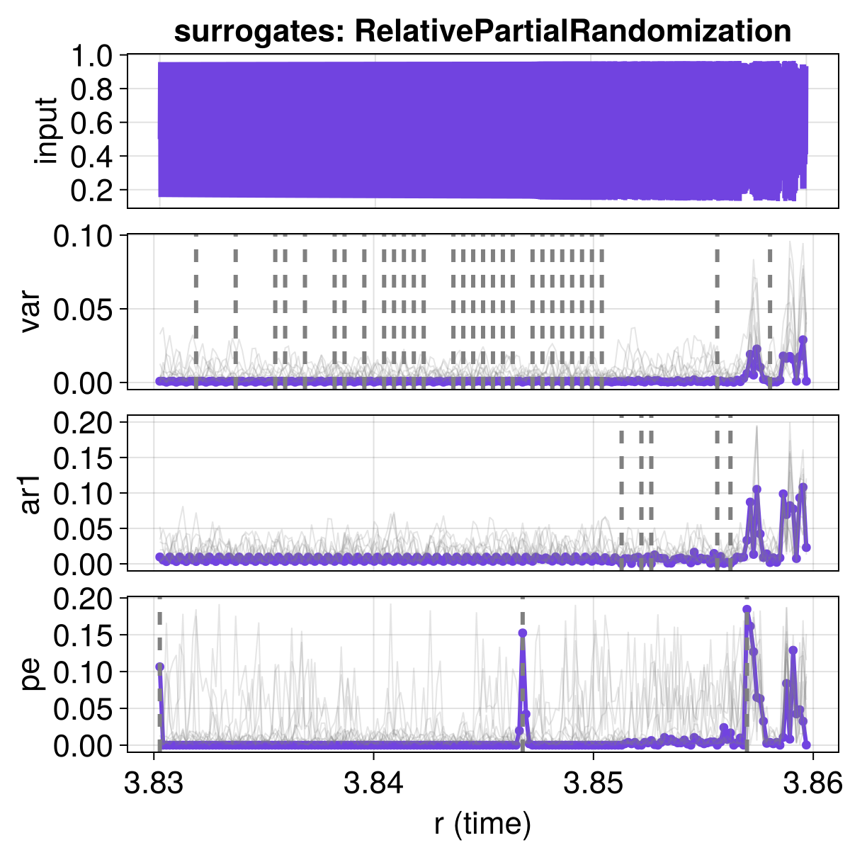

Our results have improved. In the permutation entropy, we see only two transitions detected as significant, which is correct: only two real dynamical transitions exist in the data. In the other two indicators we also see fewer transitions, but as we have already discussed, no results with the other indicators should be taken into meaningful consideration, as these indicators are simply inappropriate for what we are looking for here.

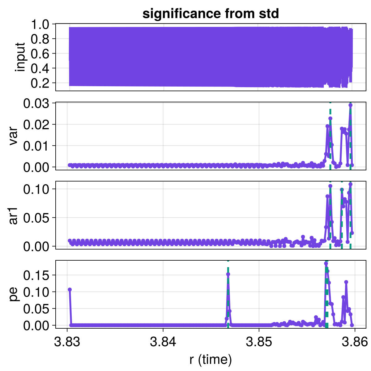
Simpler Significance

Arguably, exactly because we are using the difference_of_means as a change metric, we may want to be less strict and more simple with our tests for significance. Instead of using SurrogatesSignificance we may use the simpler and much faster SigmaSignificance, which simply claims significant time points whenever a change metric exceeds some pre-defined factor of its timeseries standard deviation.

fig = plot_change_metrics()
flags = significant_transitions(results, SigmaSignificance(factor = 5.0))

# Plot the flags
for (i, indicator) in enumerate(indicators)
    vlines!(fig[i+1, 1], results.t_change[flags[:, i]];
        color = Cycled(3), linestyle = :dash, linewidth = 3
    )
end
content(fig[1, 1]).title = "significance from std"
fig