Integrating Agents.jl with DifferentialEquations.jl
Leveraging other best-in-class packages from the Julia ecosystem is one of the many strengths Agents.jl provides over alternative ABMs.
The DifferentialEquations.jl package is one excellent example. Here, we provide a few ways of leveraging DifferentialEquations to solve agent based models in an efficient and performant manner, whilst mitigating stability issues one may encounter.
It is common in discrete time step tools (such as Agents) to also discretise equations required for obtaining solutions. In the following example, we use the forward Euler method to discretise a logistic function
$\frac{\mathrm{d}s}{\mathrm{d}t} = s \left(1-\frac{s}{120}\right) - h$
into
$s_{t+1} = s_t + s_t (1-s_t/120)-h.$
In this example, $s$ denotes some fish stock that increases over time until a maximum population (e.g. 120 here) is met, with the additional property that a harvest ($h$) may also remove some population (we also assume a timestep of 1 normalised unit to simplify things).
Problem setup
Let's build a fishing community with fishers, each with differing methods and experience, culminating in a variety of competence when it comes to actually catching fish.
using Agents
using Distributions
using CairoMakie

@agent struct Fisher(NoSpaceAgent)
    competence::Int
    yearly_catch::Float64
end

function agent_step!(agent, model)
    # Make sure we sample from the fish distribution
    return agent.yearly_catch = rand(abmrng(model), Poisson(agent.competence))
end

function dstock(model)
    # Only allow fishing if stocks are high enough
    h = model.stock > model.min_threshold ? sum(a.yearly_catch for a in allagents(model)) :
        0.0

    return model.stock * (1 - (model.stock / model.max_population)) - h
end

function model_step!(model)
    return model.stock += dstock(model)
end
These methods should be quite straightforward: each step of the model (agent_step!), every agent will catch some fish based on their competency. There are some safeguards in place to not allow fishers to totally deplete the stock, thus dstock checks the total yearly catch and only harvests if the population is above a minimal threshold (in a more complete example, one should set a flag to state that this year's catch exceeded the limit and regulate fishing next year, but we'll ignore this complexity for this example).
Building this model is simple. Set some initial conditions for the stock, and add agents with some competence.
function initialise(;
        stock = 5.0, # Initial population of fish
        max_population = 500.0, # Maximum value of fish stock
        min_threshold = 60.0, # Regulate fishing if population drops below this value
        nagents = 50,
    )
    model = StandardABM(
        Fisher;
        agent_step!,
        model_step!,
        properties = Dict(
            :stock => stock,
            :max_population => max_population,
            :min_threshold => min_threshold,
        ),
    )
    for _ in 1:nagents
        add_agent!(
            model,
            # Competence level is a lognormal distribution between 1 and 5
            floor(rand(abmrng(model), truncated(LogNormal(), 1, 6))),
            # Yearly catch can start at 0
            0.0,
        )
    end
    return model
end
We can now run the model and see how the fishery fairs over the next 20 years.
model = initialise()
_, results = run!(model, 20; mdata = [:stock])

f = Figure(size = (600, 400))
ax = f[1, 1] = Axis(
    f,
    xlabel = "Year",
    ylabel = "Stock",
    title = "Fishery Inventory",
)
lines!(ax, results.stock, linewidth = 2, color = :blue)
f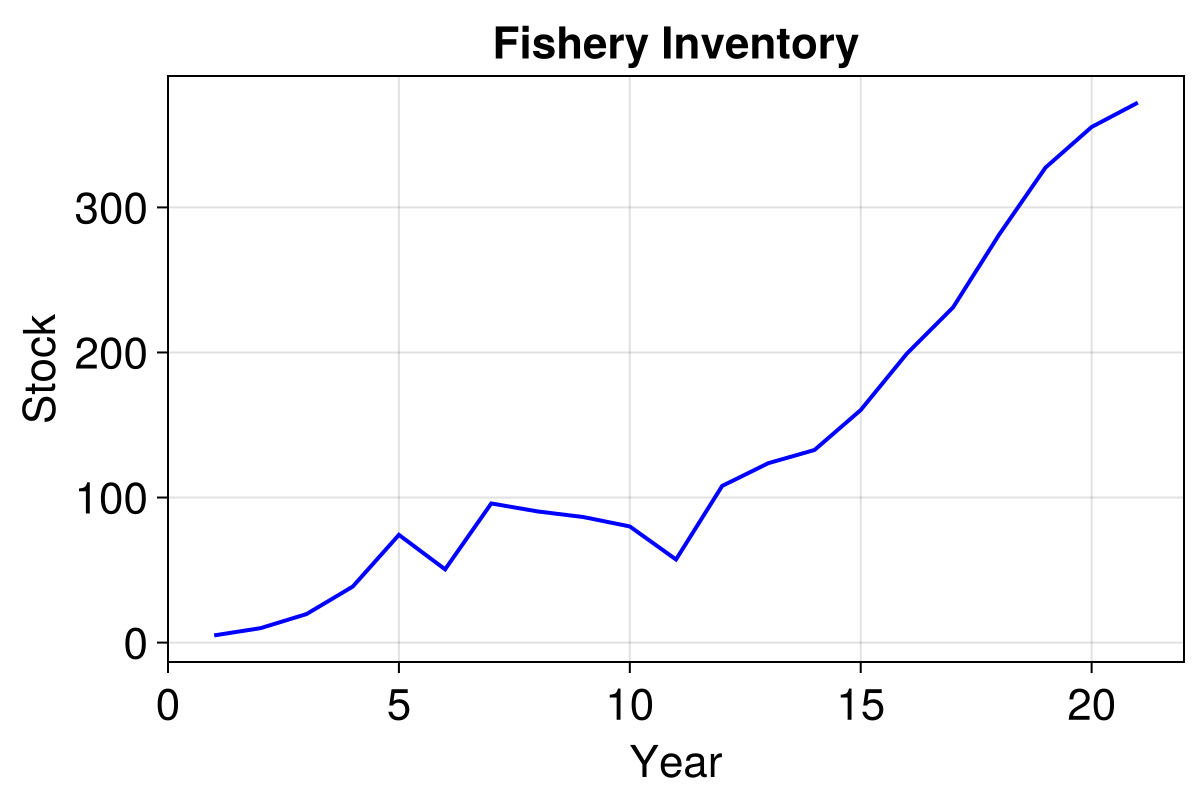
Add in some bureaucracy
OK, so let's add in some annoyances for the fishers. Of course, they wish to go out and catch regularly, but regulators only want to do their job once a year! Since it's the regulators who will monitor the total stock condition and advise fishers as to whether or not they can continue fishing, a systematic blind spot is inadvertently introduced into the system. Yearly catch and regulation occur on one day a year, whilst the stock will of course grow on a daily basis.
To achieve this, we extend the model like so:
function agent_step!(agent, model)
    return if model.tick % 365 == 0
        agent.yearly_catch = rand(abmrng(model), Poisson(agent.competence))
    end
end

function dstock(model)
    # Only allow fishing if stocks are high enough
    # (monitored yearly, so this will return 0 364 days of the year)
    h = model.tick % 365 == 0 && model.stock > model.min_threshold ?
        sum(a.yearly_catch for a in allagents(model)) : 0.0

    return model.stock * (1 - (model.stock / model.max_population)) - h
end

function model_step!(model)
    model.tick += 1
    return model.stock += dstock(model)
end

function initialise(;
        stock = 400.0, # Initial population of fish (lets move to an equilibrium position)
        max_population = 500.0, # Maximum value of fish stock
        min_threshold = 60.0, # Regulate fishing if population drops below this value
        nagents = 50,
    )
    model = StandardABM(
        Fisher;
        agent_step!,
        model_step!,
        properties = Dict(
            :stock => stock,
            :max_population => max_population,
            :min_threshold => min_threshold,
            :tick => 0, # Time keeper in units of days
        ),
    )
    for _ in 1:nagents
        add_agent!(model, floor(rand(abmrng(model), truncated(LogNormal(), 1, 6))), 0.0)
    end
    return model
end
Now that our model is running with a daily timestep, we must extend the run length value, and we'll also start from a steady state population.
model = initialise()
yearly(model, s) = s % 365 == 0
_, results = run!(model, 20 * 365; mdata = [:stock], when = yearly)

f = Figure(size = (600, 400))
ax = Axis(
    f[1, 1],
    xlabel = "Year",
    ylabel = "Stock",
    title = "Fishery Inventory",
)
lines!(ax, results.stock, linewidth = 2, color = :blue)
f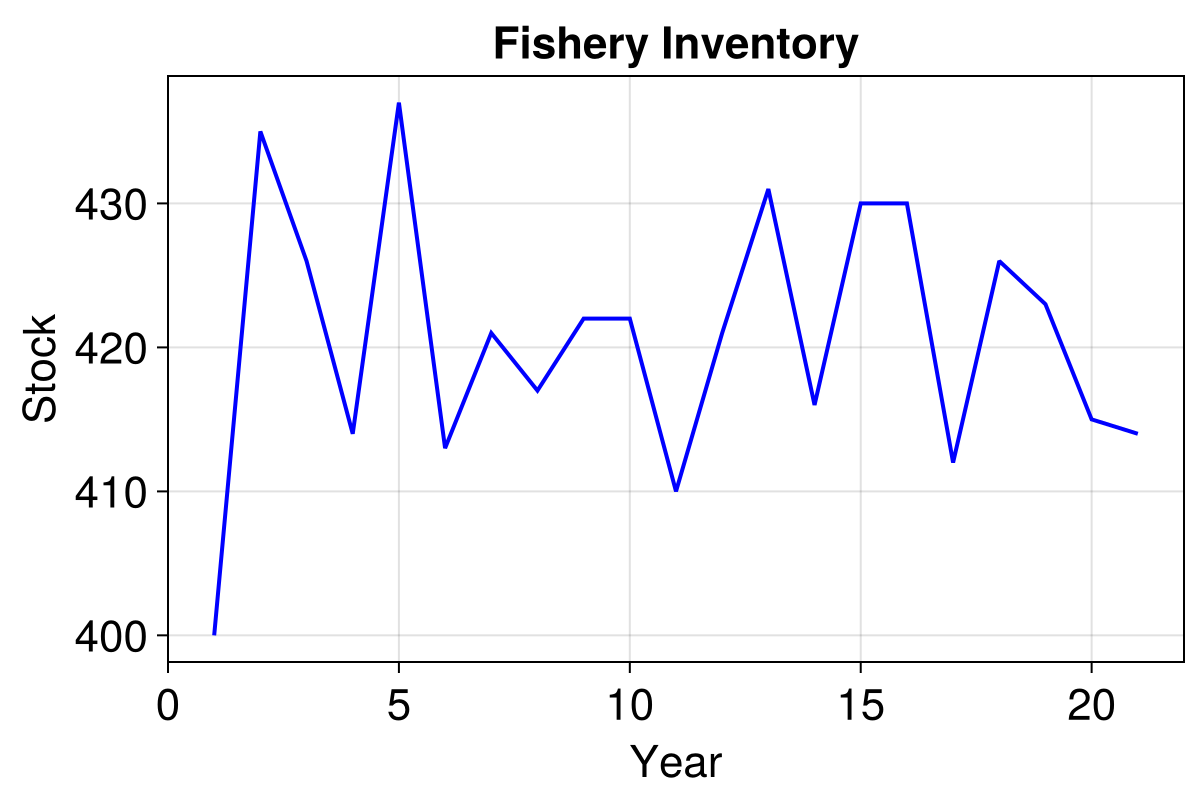
Baseline benchmark
Lets get a baseline performance result for our model.
using BenchmarkTools

@btime Agents.step!(model, 20 * 365) setup = (model = initialise())
StandardABM with 50 agents of type Fisher
agents container: Dict
space: nothing (no spatial structure)
scheduler: fastest
properties: stock, min_threshold, tick, max_populationSo this is fairly quick since the model is a simple one, but it's certainly not as efficient as it could be. We calculate the stock value every single day, since the forward Eulerian method requires us to, so it can evolve correctly. In addition to this, Eulerian expansion introduces uncertainty into our results, which is tied to the choice of step size. For accurate results, one should never really use this approximate method - although it is almost ubiquitous throughout contemporary research code. For a thorough exposé on this, have a read of Why you shouldn't use Euler's method to solve ODEs.
Coupling DifferentialEquations.jl to Agents.jl
Lets therefore modify our system to solve the logistic equation in a continuous context, but discretely monitor and harvest.
import OrdinaryDiffEqTsit5

function agent_diffeq_step!(agent, model)
    return agent.yearly_catch = rand(abmrng(model), Poisson(agent.competence))
end

function model_diffeq_step!(model)
    # We step 364 days with this call.
    OrdinaryDiffEqTsit5.step!(model.i, 364.0, true)
    # Only allow fishing if stocks are high enough
    model.i.p[2] =
        model.i.u[1] > model.min_threshold ? sum(a.yearly_catch for a in allagents(model)) :
        0.0
    # Notify the integrator that conditions may be altered
    OrdinaryDiffEqTsit5.u_modified!(model.i, true)
    # Then apply our catch modifier
    OrdinaryDiffEqTsit5.step!(model.i, 1.0, true)
    # Store yearly stock in the model for plotting
    model.stock = model.i.u[1]
    # And reset for the next year
    model.i.p[2] = 0.0
    return OrdinaryDiffEqTsit5.u_modified!(model.i, true)
end

function initialise_diffeq(;
        stock = 400.0, # Initial population of fish (lets move to an equilibrium position)
        max_population = 500.0, # Maximum value of fish stock
        min_threshold = 60.0, # Regulate fishing if population drops below this value
        nagents = 50,
    )

    function fish_stock!(ds, s, p, t)
        max_population, h = p
        return ds[1] = s[1] * (1 - (s[1] / max_population)) - h
    end
    prob =
        OrdinaryDiffEqTsit5.ODEProblem(fish_stock!, [stock], (0.0, Inf), [max_population, 0.0])
    integrator = OrdinaryDiffEqTsit5.init(prob, OrdinaryDiffEqTsit5.Tsit5(); advance_to_tstop = true)

    model = StandardABM(
        Fisher;
        agent_step! = agent_diffeq_step!,
        model_step! = model_diffeq_step!,
        properties = Dict(
            :stock => stock,
            :max_population => max_population,
            :min_threshold => min_threshold,
            :i => integrator, # The OrdinaryDiffEqTsit5 integrator
        ),
    )
    for _ in 1:nagents
        add_agent!(model, floor(rand(abmrng(model), truncated(LogNormal(), 1, 6))), 0.0)
    end
    return model
end
Notice that we've reverted back to a yearly rather than daily timestep here, since the ODE solver is now in charge of evolving the logistic function forward. We've used the integrator interface to achieve this.
Note that we use OrdinaryDiffEqTsit5 here, which is a component of DifferentialEquations.jl Users may switch this to any subcomponent of the DifferentialEquations.jl ecosystem.
This implementation uses import to explicitly identify which functions are from OrdinaryDiffEqTsit5 and not Agents. However, since both Agents and OrdinaryDiffEqTsit5 provide a step! function, each use must be qualified explicitly if one were to choose to bring all of DifferentialEquations into scope via the using keyword.
modeldeq = initialise_diffeq()
_, resultsdeq = run!(modeldeq, 20; mdata = [:stock])

f = Figure(size = (600, 400))
ax = Axis(
    f[1, 1];
    xlabel = "Year",
    ylabel = "Stock",
    title = "Fishery Inventory",
)
lines!(ax, resultsdeq.stock, linewidth = 2, color = :blue)
f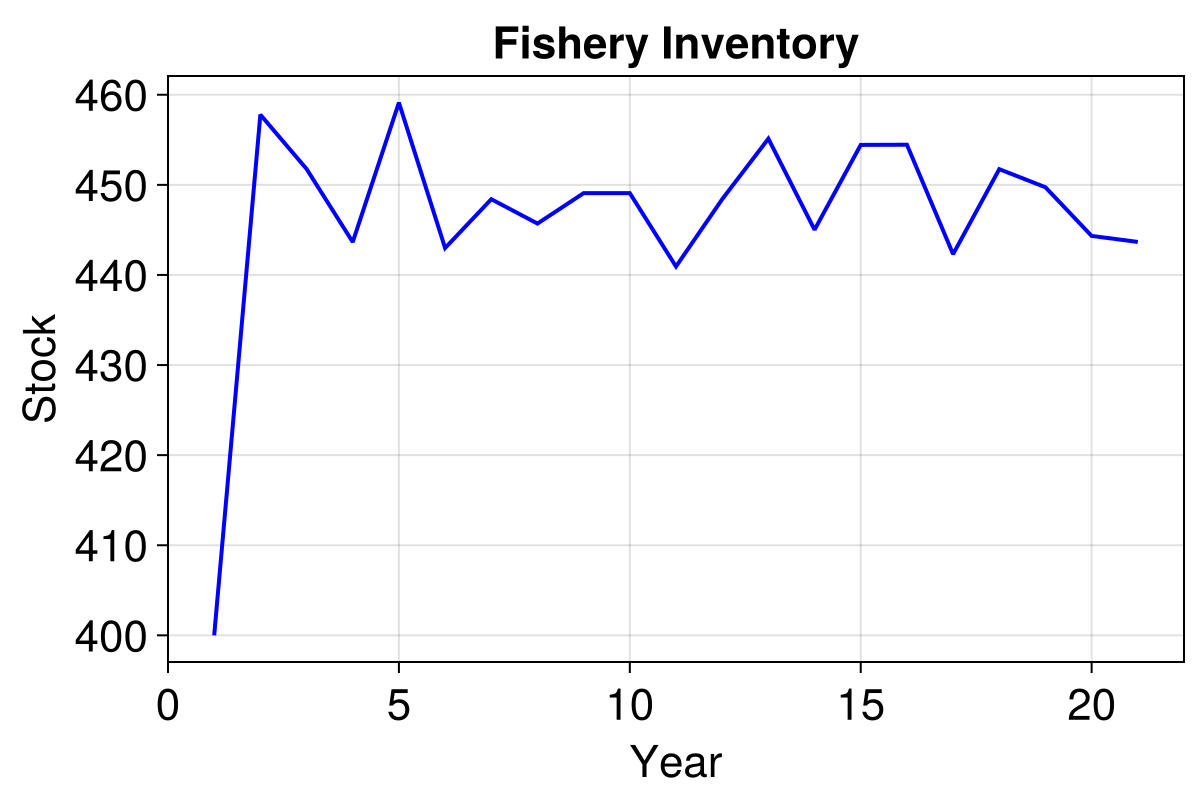
The small complexity addition yields us a generous speed up of around 4.5x.
@btime Agents.step!(model, 20) setup = (model = initialise_diffeq())StandardABM with 50 agents of type Fisher
agents container: Dict
space: nothing (no spatial structure)
scheduler: fastest
properties: stock, min_threshold, i, max_populationDigging into the results a little more, we can see that the DifferentialEquations solver did not need to solve the logistic equation at every agent step to achieve a stable solution for us:
length(modeldeq.i.sol.t)2191365 * 20 > length(modeldeq.i.sol.t)trueWith other initial conditions, there's the possibility that this may not be the case. When this occurs, these additional samples provide mathematical guarantees that the results are accurate (to a given tolerance), which is a safeguard not possible for our Euler example.
Compare our two results directly, both start with the same random seed and evolve in precisely the same manner:
f = Figure(size = (600, 400))
ax = Axis(
    f[1, 1];
    xlabel = "Year",
    ylabel = "Stock",
    title = "Fishery Inventory",
)
lineE = lines!(ax, results.stock, linewidth = 2, color = :blue)
lineTS = lines!(ax, resultsdeq.stock, linewidth = 2, color = :red)
leg = f[1, end + 1] = Legend(f, [lineE, lineTS], ["Euler", "TSit5"])
f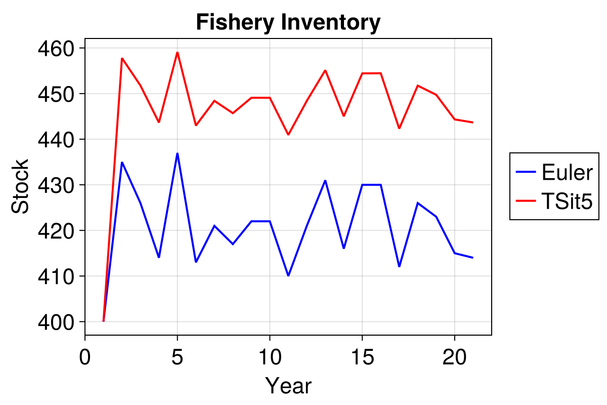
That's an average discrepancy of 30 fish! Optimising the step size in the Euler method can close this gap, but this is yet more analysis overhead we'd prefer to avoid by using better solutions.
In addition, the ODE solver will be faster most of the time, regardless of how many steps it needs to take. If not, there are other, more effective solvers that can be used for your particular case.
Coupling Agents.jl to DifferentialEquations.jl
Perhaps you're more familiar to the DifferentialEquations solve interface and you're new to Agents?
We can also couple the two systems the other way. Let's use callbacks to handle the agent based aspects of our problem.
function agent_cb_step!(agent, model)
    return agent.yearly_catch = rand(abmrng(model), Poisson(agent.competence))
end

function initialise_cb(; min_threshold = 60.0, nagents = 50)
    model = StandardABM(
        Fisher; agent_step! = agent_cb_step!,
        properties = Dict(:min_threshold => min_threshold)
    )
    for _ in 1:nagents
        add_agent!(model, floor(rand(abmrng(model), truncated(LogNormal(), 1, 6))), 0.0)
    end
    return model
end

modelcb = initialise_cb()
StandardABM with 50 agents of type Fisher
agents container: Dict
space: nothing (no spatial structure)
scheduler: fastest
properties: min_thresholdThat's it for the Agents side of things! Now to build the ODE.
import DiffEqCallbacks

function fish!(integrator, model)
    integrator.p[2] = integrator.u[1] > model.min_threshold ?
        sum(a.yearly_catch for a in allagents(model)) : 0.0
    return Agents.step!(model, 1)
end

function fish_stock!(ds, s, p, t)
    max_population, h = p
    return ds[1] = s[1] * (1 - (s[1] / max_population)) - h
end

tspan = (0.0, 20.0 * 365.0)
const initial_stock = 400.0
const max_population = 500.0

prob = OrdinaryDiffEqTsit5.ODEProblem(fish_stock!, [initial_stock], tspan, [max_population, 0.0])

# Each Dec 31st, we call fish! that adds our catch modifier to the stock, and steps the model
fish = DiffEqCallbacks.PeriodicCallback(i -> fish!(i, modelcb), 364)
# Stocks are replenished again
reset = DiffEqCallbacks.PeriodicCallback(i -> i.p[2] = 0.0, 365)

sol = OrdinaryDiffEqTsit5.solve(
    prob,
    OrdinaryDiffEqTsit5.Tsit5();
    callback = OrdinaryDiffEqTsit5.CallbackSet(fish, reset),
)
discrete = vcat(sol(0:365:(365 * 20))[:, :]...)
fig = Figure(size = (600, 400))
ax = Axis(
    fig[1, 1];
    xlabel = "Year",
    ylabel = "Stock",
    title = "Fishery Inventory",
)
lines!(ax, discrete, linewidth = 2, color = :blue)
fig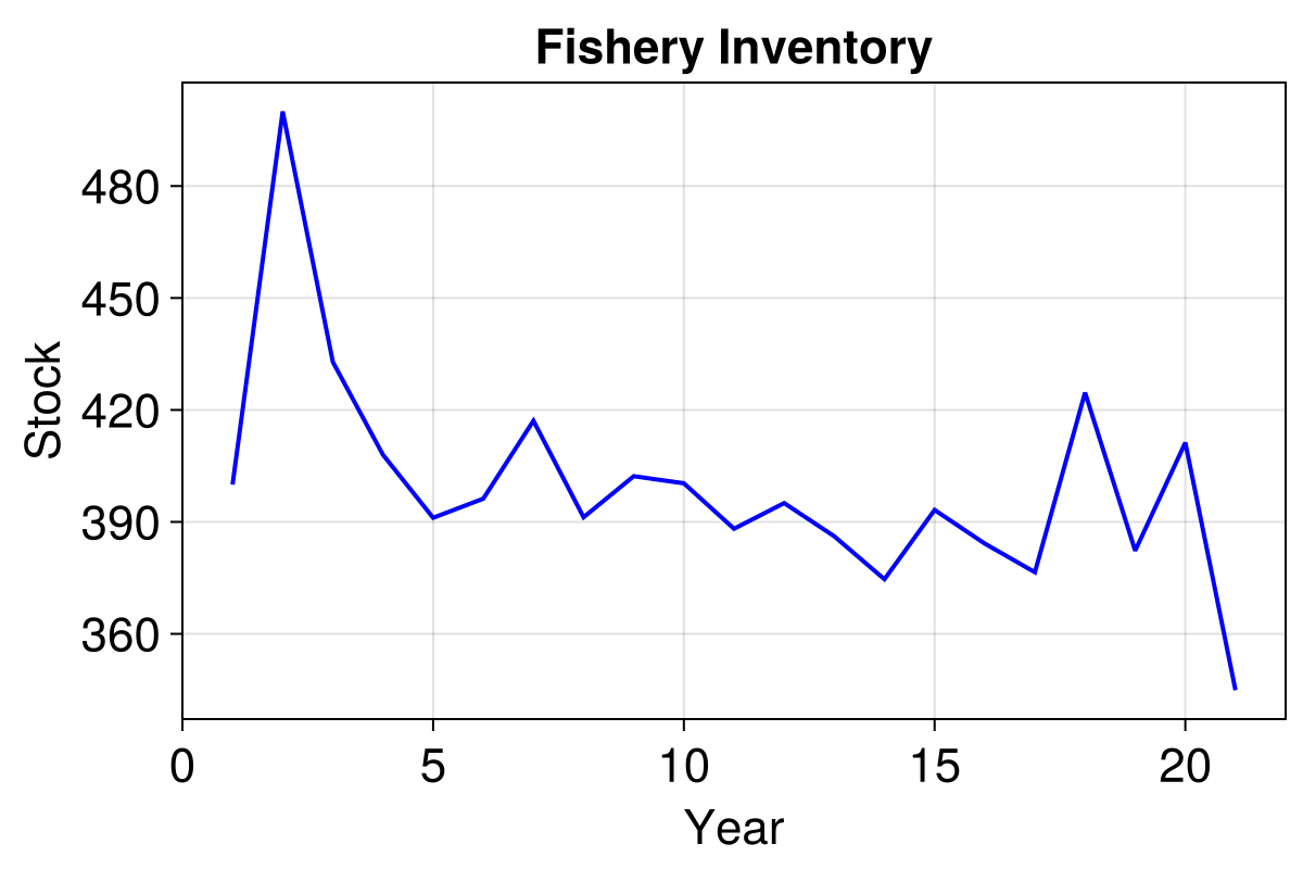
The results are different here, since the construction of this version and the one above are quite different and cannot be randomly seeded in the same manner.
However, as you can see, it is for the most part just a re-arranged implementation of the integrator method - giving users flexibility in their architecture choices.