SIR model for the spread of COVID-19
This example illustrates how to use GraphSpace and how to model agents moving on a graph (network) where the transition probabilities between each node (position) is not constant.
SIR model
A SIR model tracks the ratio of Susceptible, Infected, and Recovered individuals within a population. Here we add one more category of individuals: those who are infected, but do not know it. Transmission rate for infected and diagnosed individuals is lower than infected and undetected. We also allow a fraction of recovered individuals to catch the disease again, meaning that recovering the disease does not bring full immunity.
Model parameters
Here are the model parameters, some of which have default values.
Ns: a vector of population sizes per city. The amount of cities is justC=length(Ns).β_und: a vector for transmission probabilities β of the infected but undetected per city. Transmission probability is how many susceptible are infected per day by an infected individual. If social distancing is practiced, this number decreases.β_det: an array for transmission probabilities β of the infected and detected per city. If hospitals are full, this number increases.infection_period = 30: how many days before a person dies or recovers.detection_time = 14: how many days before an infected person is detected.death_rate = 0.02: the probability that the individual will die after theinfection_period.reinfection_probability = 0.05: The probability that a recovered person can get infected again.migration_rates: A matrix of migration probability per individual per day from one city to another.Is = [zeros(C-1)..., 1]: An array for initial number of infected but undetected people per city. This starts as only one infected individual in the last city.
Notice that Ns, β, Is all need to have the same length, as they are numbers for each city. We've tried to add values to the infection parameters similar to the ones you would hear on the news about COVID-19.
The good thing with Agent based models is that you could easily extend the model we implement here to also include age as an additional property of each agent. This makes ABMs flexible and suitable for research of virus spreading.
Making the model in Agents.jl
We start by defining the PoorSoul agent type and the ABM
using Agents, Random
using Agents.DataFrames, Agents.Graphs
using StatsBase: sample, Weights
using DrWatson: @dict
using CairoMakie

@agent struct PoorSoul(GraphAgent)
    days_infected::Int  # number of days since is infected
    status::Symbol  # 1: S, 2: I, 3:R
end

function model_initiation(;
        Ns,
        migration_rates,
        β_und,
        β_det,
        infection_period = 30,
        reinfection_probability = 0.05,
        detection_time = 14,
        death_rate = 0.02,
        Is = [zeros(Int, length(Ns) - 1)..., 1],
        seed = 0,
    )

    rng = Xoshiro(seed)
    @assert length(Ns) ==
        length(Is) ==
        length(β_und) ==
        length(β_det) ==
        size(migration_rates, 1) "length of Ns, Is, and B, and number of rows/columns in migration_rates should be the same "
    @assert size(migration_rates, 1) == size(migration_rates, 2) "migration_rates rates should be a square matrix"

    C = length(Ns)
    # normalize migration_rates
    migration_rates_sum = sum(migration_rates, dims = 2)
    for c in 1:C
        migration_rates[c, :] ./= migration_rates_sum[c]
    end

    properties = @dict(
        Ns,
        Is,
        β_und,
        β_det,
        β_det,
        migration_rates,
        infection_period,
        infection_period,
        reinfection_probability,
        detection_time,
        C,
        death_rate,
    )
    space = GraphSpace(complete_graph(C))
    model = StandardABM(PoorSoul, space; agent_step!, properties, rng)

    # Add initial individuals
    for city in 1:C, n in 1:Ns[city]
        ind = add_agent!(city, model, 0, :S) # Susceptible
    end
    # add infected individuals
    for city in 1:C
        inds = ids_in_position(city, model)
        for n in 1:Is[city]
            agent = model[inds[n]]
            agent.status = :I # Infected
            agent.days_infected = 1
        end
    end
    return model
end
model_initiation (generic function with 1 method)We will make a function that starts a model with C number of cities, and creates the other parameters automatically by attributing some random values to them. You could directly use the above constructor and specify all Ns, β, etc. for a given set of cities.
All cities are connected with each other, while it is more probable to travel from a city with small population into a city with large population.
using LinearAlgebra: diagind

function create_params(;
        C,
        max_travel_rate,
        infection_period = 30,
        reinfection_probability = 0.05,
        detection_time = 14,
        death_rate = 0.02,
        Is = [zeros(Int, C - 1)..., 1],
        seed = 19,
    )

    Random.seed!(seed)
    Ns = rand(50:500, C)
    β_und = rand(0.3:0.02:0.6, C)
    β_det = β_und ./ 10

    Random.seed!(seed)
    migration_rates = zeros(C, C)
    for c in 1:C
        for c2 in 1:C
            migration_rates[c, c2] = (Ns[c] + Ns[c2]) / Ns[c]
        end
    end
    maxM = maximum(migration_rates)
    migration_rates = (migration_rates .* max_travel_rate) ./ maxM
    migration_rates[diagind(migration_rates)] .= 1.0

    params = @dict(
        Ns,
        β_und,
        β_det,
        migration_rates,
        infection_period,
        reinfection_probability,
        detection_time,
        death_rate,
        Is
    )

    return params
end
create_params (generic function with 1 method)SIR Stepping functions
Now we define the functions for modelling the virus spread in time
function agent_step!(agent, model)
    migrate!(agent, model)
    transmit!(agent, model)
    update!(agent, model)
    return recover_or_die!(agent, model)
end

function migrate!(agent, model)
    pid = agent.pos
    m = sample(abmrng(model), 1:(model.C), Weights(model.migration_rates[pid, :]))
    if m ≠ pid
        move_agent!(agent, m, model)
    end
    return
end

function transmit!(agent, model)
    agent.status == :S && return
    rate = if agent.days_infected < model.detection_time
        model.β_und[agent.pos]
    else
        model.β_det[agent.pos]
    end

    n = rate * abs(randn(abmrng(model)))
    n <= 0 && return

    for contactID in ids_in_position(agent, model)
        contact = model[contactID]
        if contact.status == :S ||
                (contact.status == :R && rand(abmrng(model)) ≤ model.reinfection_probability)
            contact.status = :I
            n -= 1
            n <= 0 && return
        end
    end
    return
end

update!(agent, model) = agent.status == :I && (agent.days_infected += 1)

function recover_or_die!(agent, model)
    return if agent.days_infected ≥ model.infection_period
        if rand(abmrng(model)) ≤ model.death_rate
            remove_agent!(agent, model)
        else
            agent.status = :R
            agent.days_infected = 0
        end
    end
end

params = create_params(C = 8, max_travel_rate = 0.01)
model = model_initiation(; params...)
StandardABM with 2960 agents of type PoorSoul
agents container: Dict
space: GraphSpace with 8 positions and 28 edges
scheduler: fastest
properties: Is, death_rate, infection_period, β_und, Ns, migration_rates, detection_time, reinfection_probability, β_det, CVisualizing GraphSpaces
GraphSpaces can be visualized by leveraging the GraphMakie.jl package. Plotting for such spaces is handled a bit differently though. Normally the agent_color, agent_size, agent_marker keyword arguments generally relate to agent colors, markersizes, and markers. For GraphSpaces, they collect those plot attributes for each node of the underlying graph which can contain multiple agents. So the function given to agent_color inputs an iterable of agents.
In this model, we color each cite according to the infected population and make the marker size proportional to the population. And remember, the package GraphMakie must be in scope for this plotting to work!
using GraphMakie
city_size(agents_here) = 0.1 * length(agents_here)
function city_color(agents_here)
    l_agents_here = length(agents_here)
    infected = count(a.status == :I for a in agents_here)
    recovered = count(a.status == :R for a in agents_here)
    return Makie.RGB(infected / l_agents_here, recovered / l_agents_here, 0)
end
city_color (generic function with 1 method)Since the underlying graph will be visualized we have the power to also style how the edges of the graph will be plotted. We do this through the keywordagentsplotkwargs of abmplot, which contains options that will be propagated to GraphMakie.graphplot. Special keywords there are edge_color, edge_width, both of which can be functions inputting the model and outputting a vector with the same length (or twice) as current number of edges in the underlying graph, to style the color and width of the edges.
edge_color(model) = fill((:grey, 0.5), ne(abmspace(model).graph))
function edge_width(model)
    w = zeros(ne(abmspace(model).graph))
    for e in edges(abmspace(model).graph)
        w[e.src] = 0.002 * length(abmspace(model).stored_ids[e.src])
        w[e.dst] = 0.002 * length(abmspace(model).stored_ids[e.dst])
    end
    return w
end

agentsplotkwargs = (
    layout = GraphMakie.Shell(), # node positions layout
    arrow_show = false, # hide directions of graph edges
    edge_color = edge_color, # change edge colors and widths with own functions
    edge_width = edge_width,
    edge_plottype = :linesegments, # needed for tapered edge widths
)
(layout = NetworkLayout.Shell{Float64}(Vector{Int64}[]), arrow_show = false, edge_color = Main.edge_color, edge_width = Main.edge_width, edge_plottype = :linesegments)we now put everything together:
fig, ax, abmobs = abmplot(
    model;
    agent_size = city_size, agent_color = city_color, agentsplotkwargs
)
fig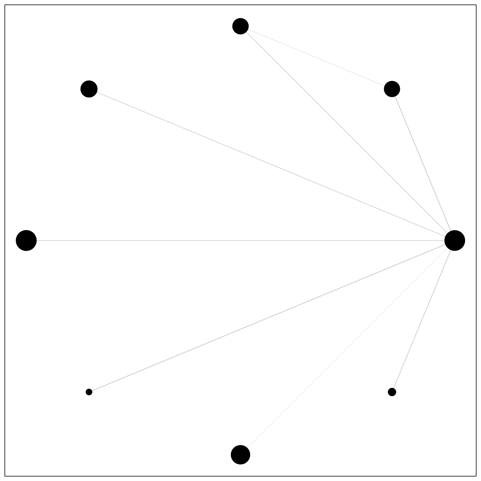
Naturally, animating the evolution of this model through abmvideo is the same as any other example:
abmvideo(
    "covid_evolution.mp4", model;
    agent_size = city_size, agent_color = city_color, agentsplotkwargs,
    framerate = 4, frames = 25,
    title = "SIR model for COVID-19 spread"
)
One can really see "explosive growth" in this animation. Things look quite calm for a while and then suddenly supermarkets have no toilet paper anymore!
Exponential growth
This observation is characterized by the exponential growth in the number of infected. We now run the model and collect data to quantify this. We define two useful functions for data collection:
infected(x) = count(i == :I for i in x)
recovered(x) = count(i == :R for i in x)
recovered (generic function with 1 method)and then collect data
model = model_initiation(; params...)

to_collect = [(:status, f) for f in (infected, recovered, length)]
data, _ = run!(model, 50; adata = to_collect)
data[1:10, :]| Row | time | infected_status | recovered_status | length_status |
|---|---|---|---|---|
| Int64 | Int64 | Int64 | Int64 | |
| 1 | 0 | 1 | 0 | 2960 |
| 2 | 1 | 3 | 0 | 2960 |
| 3 | 2 | 15 | 0 | 2960 |
| 4 | 3 | 38 | 0 | 2960 |
| 5 | 4 | 127 | 0 | 2960 |
| 6 | 5 | 279 | 0 | 2960 |
| 7 | 6 | 430 | 0 | 2960 |
| 8 | 7 | 846 | 0 | 2960 |
| 9 | 8 | 1943 | 0 | 2960 |
| 10 | 9 | 2936 | 0 | 2960 |
We now plot how quantities evolved in time to show the exponential growth of the virus
N = sum(model.Ns) # Total initial population
fig = Figure(size = (600, 400))
ax = fig[1, 1] = Axis(fig, xlabel = "steps", ylabel = "log10(count)")
li = lines!(ax, data.time, log10.(data[:, dataname((:status, infected))]), color = :blue)
lr = lines!(ax, data.time, log10.(data[:, dataname((:status, recovered))]), color = :red)
dead = log10.(N .- data[:, dataname((:status, length))])
ld = lines!(ax, data.time, dead, color = :green)
Legend(fig[1, 2], [li, lr, ld], ["infected", "recovered", "dead"])
fig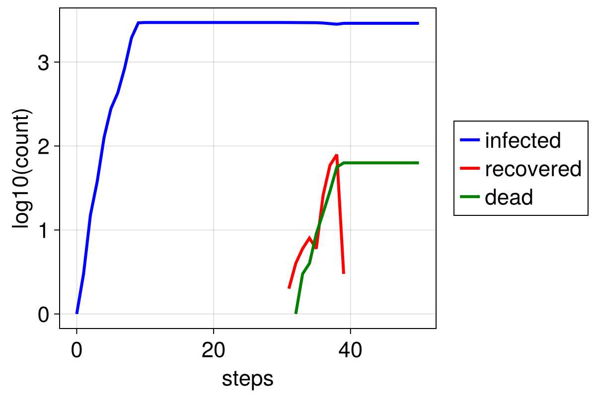
The exponential growth is clearly visible since the logarithm of the number of infected increases linearly, until everyone is infected.