Tutorial

This is the main overarching tutorial for Agents.jl. It will walk you through the typical workflow of doing agent based modelling (ABM) using Agents.jl, while introducing and explaining the core components of Agents.jl. The tutorial will utilize the Schelling segregation model as an example to apply the concepts we learn.

Besides the normal step-by-step educative version of the tutorial, there is also the fast, shortened, copy-pasteable version right below. We strongly recommend going through the normal tutorial step-by-step though!

Tutorial - copy-pasteable version

Gotta go fast!

using Agents # bring package into scope

# make the space the agents will live in
space = GridSpace((20, 20)) # 20×20 grid cells

# make an agent type appropriate to this space and with the
# properties we want based on the ABM we will simulate
@agent struct Schelling(GridAgent{2}) # inherit all properties of `GridAgent{2}`
    mood::Bool = false # all agents are sad by default :'(
    group::Int # the group does not have a default value!
end

# define the evolution rule: a function that acts once per step on
# all activated agents (acts in-place on the given agent)
function schelling_step!(agent, model)
    # Here we access a model-level property `min_to_be_happy`
    # This will have an assigned value once we create the model
    minhappy = model.min_to_be_happy
    count_neighbors_same_group = 0
    # For each neighbor, get group and compare to current agent's group
    # and increment `count_neighbors_same_group` as appropriately.
    # Here `nearby_agents` (with default arguments) will provide an iterator
    # over the nearby agents one grid cell away, which are at most 8.
    for neighbor in nearby_agents(agent, model)
        if agent.group == neighbor.group
            count_neighbors_same_group += 1
        end
    end
    # After counting the neighbors, decide whether or not to move the agent.
    # If `count_neighbors_same_group` is at least min_to_be_happy, set the
    # mood to true. Otherwise, move the agent to a random position, and set
    # mood to false.
    if count_neighbors_same_group ≥ minhappy
        agent.mood = true
    else
        agent.mood = false
        move_agent_single!(agent, model)
    end
    return
end

# make a container for model-level properties
properties = Dict(:min_to_be_happy => 3)

# Create the central `AgentBasedModel` that stores all simution information
model = StandardABM(
    Schelling, # type of agents
    space; # space they live in
    agent_step! = schelling_step!, properties
)

# populate the model with agents by automatically creating and adding them
# to random position in the space
for n in 1:300
    add_agent_single!(model; group = n < 300 / 2 ? 1 : 2)
end

# run the model for 5 steps, and collect data.
# The data to collect are given as a vector of tuples: 1st element of tuple is
# what property, or what function of agent -> data, to collect. 2nd element
# is how to aggregate the collected property over all agents in the simulation
using Statistics: mean
xpos(agent) = agent.pos[1]
adata = [(:mood, sum), (xpos, mean)]
adf, mdf = run!(model, 5; adata)
adf # a Julia `DataFrame`

Core steps of an Agents.jl simulation

In Agents.jl a central abstract structure called AgentBasedModel contains all information necessary to run a simulation: the evolution rule (also called dynamic rule), the agents of the simulation, the space the agents move and interact in, and other model-level properties relevant to the simulation.

An Agents.jl simulation is composed of first building such an AgentBasedModel (steps 1-4 below) and then evolving it and/or analyzing it (steps 5-7 below):

1. Choose what kind of space the agents will live in, for example a graph, a grid, etc. Several spaces are provided by Agents.jl and can be initialized immediately.
2. Define the agent type(s) that will populate the ABM. Agent types are Julia mutable structs that are created with @agent. The types must contain some mandatory fields, which is ensured by using @agent. The remaining fields of the agent type are up to the user's choice.
3. Define the evolution rule(s), i.e., how the model evolves in time. The evolution rule(s) are always standard Julia functions that take advantage of the Agents.jl API. The exact way one defines the evolution rules depends on the type of AgentBasedModel used. Agents.jl allows simulations in both discrete time via StandardABM as well as continuous time via EventQueueABM. In this tutorial we will learn the discrete-time version. See the rock-paper-scissors example for an introduction to the continuous time version.
4. Initialize an AgentBasedModel instance that contains the agent type(s), the chosen space, the evolution rule(s), other optional additional model-level properties, and other simulation tuning properties like schedulers or random number generators. Then, populate this model with agent instances.
5. (Trivial) evolve the model forwards in time.
6. (Optional) Visualize the model and animate its time evolution. This can help checking that the model behaves as expected and there aren't any mistakes, or can be used in making figures for a paper/presentation.
7. Collect data. To do this, specify which data should be collected, by providing one standard Julia Vector of data-to-collect for agents, for example [:mood, :wealth], and another one for the model. The agent data names are given as the keyword adata and the model as keyword mdata to the function run!. This function outputs collected data in the form of a DataFrame.

In the spirit of simple design, all of these steps are done by defining simple Julia data structures, like vectors, dictionaries, functions, or structs. This means that using Agents.jl comes with transferrable knowledge to the whole Julia ecosystem. Indeed, looking at the "Integration examples" (see sidebar of online docs) Agents.jl can be readily used with any other Julia package, exactly because its design is based on existing, and widely established, Julia language concepts.

The Schelling segregation model basic rules

• A fixed pre-determined number of agents exist in the model.
• Agents belong to one of two groups (1 or 2).
• The agents live in a two-dimensional non-periodic grid.
• Only one agent per position is allowed.
• At each state of the simulation, each agent looks at its 8 neighboring positions (cardinal and diagonal directions). It then counts how many neighboring agents belong to the same group (if any). This leads to 8 neighboring positions per position (except at the edges of the grid).
• If an agent has at least min_to_be_happy neighbors belonging to the same group, then it becomes happy.
• Else, the agent is unhappy and moves to a new random location in space while respecting the 1-agent-per-position rule.

In the following we will build this model following the aforementioned steps. The 0-th step of any Agents.jl simulation is to bring the package into scope:

using Agents

Step 1: creating the space

Agents.jl offers multiple spaces one can utilize to perform simulations, all of which are listed in the available spaces section. If we go through the list, we quickly realize that the space we need to use here is GridSpaceSingle which is a grid that allows only one agent per position. So, we can go ahead and create an instance of this type. We need to specify the total size of the grid, and also that the distance metric should be the Chebyshev one, which means that diagonal and orthogonal directions quantify as the same distance away. We also specify that the space should not be periodic.

size = (10, 10)
space = GridSpaceSingle(size; periodic = false, metric = :chebyshev)

GridSpaceSingle with size (10, 10), metric=chebyshev, periodic=false

Step 2: the @agent command

Agents in Agents.jl are instances of user-defined structs that subtype AbstractAgent. This means that agents are data containers that contain some particular data fields that are necessary to perform simulations with Agents.jl, as well as any other data field that the user requires. If an agent instance agent exists in the simulation then the data field named "weight" is obtained from the agent using agent.weight. This is standard Julia syntax to access the data field named "weight" for any data structure that contains such a field.

To create agent types, and define what properties they should have, it is strongly recommended to use the @agent command. You can read its documentation in detail if you wish to understand it deeply. But the long story made sort is that this command ensures that agents have the minimum amount of required necessary properties to function within a given space and model by "inheriting" pre-defined agent properties suited for each type of space.

The simplest syntax of [@agent] is (and see its documentation for all its capabilities):

@agent struct YourAgentType(AgentTypeToInheritFrom) [<: OptionalSupertype]
    extra_property::Float64 # annotating the type leads to optimal computational performance
    other_extra_property_with_default::Bool = true
    const other_extra_constant_property::Int
    # etc...
end

The command may seem intimidating at first, but it is in truth not that different from Julia's native struct definition! For example,

@agent struct Person(GridAgent{2})
    age::Int
    money::Float64
end

would make an agent type with named properties age, money, while also inheriting all named properties of the GridAgent{2} predefined type. These properties are (id::Int, pos::Tuple{Int, Int}) and are necessary for simulating agents in a two-dimensional grid space. The documentation of each space describes what pre-defined agent one needs to inherit from in the @agent command, which is how we found that we need to put GridAgent{2} there. The {2} is simply an annotation that the space is 2-dimensional, as Agents.jl allows simulations in arbitrary-dimensional spaces.

Step 2: creating the agent type

With this knowledge, let's now make the agent type for the Schelling segregation model. According to the rules of the game, the agent needs to have two auxilary properties: its mood (boolean) and the group it belongs to (integer). The agent also needs to inherit from GridAgent{2} as in the example above. So, we define:

@agent struct SchellingAgent(GridAgent{2})
    mood::Bool # whether the agent is happy in its position
    group::Int # The group of the agent, determines mood as it interacts with neighbors
end

Let's explitily print the fields of the data structure SchellingAgent that we created:

for (name, type) in zip(fieldnames(SchellingAgent), fieldtypes(SchellingAgent))
    println(name, "::", type)
end

id::Int64
pos::Tuple{Int64, Int64}
mood::Bool
group::Int64

All these fields can be accessed during the simulation, but it is important to keep in mind that id cannot be modified, and pos must never be modified directly; only through valid API functions such as move_agent!.

For example, if we initialize such an agent

example_agent = SchellingAgent(id = 1, pos = (2, 3), mood = true, group = 1)

Main.SchellingAgent(1, (2, 3), true, 1)

we can obtain

example_agent.mood

true

and set

example_agent.mood = false

false

but can't set the id:

```
example_agent.id = 2
```
```
ERROR: setfield!: const field .id of type SchellingAgent cannot be changed
Stacktrace:
 [1] setproperty!(x::SchellingAgent, f::Symbol, v::Int64)
   @ Base .\Base.jl:41
```

Step 2: redefining agent types

You will notice that it is not possible to redefine agent types using the same name as the one they were originally defined with. E.g., this will error:

@agent struct SchellingAgent(GridAgent{2})
    mood::Bool # whether the agent is happy in its position
    group::Int # The group of the agent, determines mood as it interacts with neighbors
    age::Int
end

ERROR: invalid redefinition of constant Main.SchellingAgent
Stacktrace:
 [1] macro expansion
   @ util.jl:609 [inlined]
 [2] macro expansion
   @ .julia\dev\Agents\src\core\agents.jl:210 [inlined]
 [3] top-level scope
   @ .julia\dev\Agents\docs\src\tutorial.jl:266

This is not a limitation of Agents.jl but a fundamental limitation of the Julia language that very likely will be addressed in the near future. Normally, you would need to restart your Julia session to redefine a custom struct. However, it is simpler to just do a mass rename in the text editor you use to write Julia code (for example, Ctrl+Shift+H in VSCode can do a mass rename). Change the name of the agent type to e.g., the same name ending in 2, 3, ..., and carry on, until you are happy with the final configuration. When this happens you will have to restart Julia and rename the type back to having no numeric ending. Inconvenient, but thankfully it only takes a couple of seconds to resolve!

Step 3: form of the evolution rule(s) in discrete time

The form of the evolution rule(s) depends on the type of AgentBasedModel we want to use. For the example we are following here, we will use StandardABM. For this, time is discrete. In this case, the evolution rule needs to be provided as at least one, or at most two functions: an agent stepping function, that acts on scheduled agents one by one, and/or a model stepping function, that steps the entire model as a whole. These functions are standard Julia functions that take advantage of the Agents.jl API. At each discrete step of the simulation, the agent stepping function is applied once to all scheduled agents, and the model stepping function is applied once to the model. The model stepping function may also modify arbitrarily many agents since at any point all agents of the simulation are accessible from the agent based model.

To give you an idea, here is an example of a model stepping function:

function model_step!(model)
    exchange = model.exchange # obtain the `exchange` model property
    agent = model[5] # obtain agent with ID = 5
    # Iterate over neighboring agents (within distance 1)
    for neighbor in nearby_agents(model, agent, 1)
        transfer = minimum(neighbor.money, exchange)
        agent.money += transfer
        neighbor.money -= transfer
    end
    return # function end. As it is in-place it `return`s nothing.
end

This model stepping function did not operate on all agents of the model, only on agent with ID 5 and its spatial neighbors. Typically you would want to operate on more agents, which is why Agents.jl also allows the concept of the agent stepping function. This feature enables scheduling agents automatically given some scheduling rule, skipping the agents that were scheduled to act but have been removed from the model (due to e.g., the actions of other agents), and also allows optimizations that are based on the specific type of AgentBasedModel.

Step 3: agent stepping function for the Schelling model

According to the rules of the Schelling segregation model, we don't need a model stepping function, but an agent stepping function that acts on all agents. So we define:

function schelling_step!(agent, model)
    # Here we access a model-level property `min_to_be_happy`.
    # This will have an assigned value once we create the model.
    minhappy = model.min_to_be_happy
    count_neighbors_same_group = 0
    # For each neighbor, get group and compare to current agent's group
    # and increment `count_neighbors_same_group` as appropriately.
    # Here `nearby_agents` (with default arguments) will provide an iterator
    # over the nearby agents one grid cell away, which are at most 8.
    for neighbor in nearby_agents(agent, model)
        if agent.group == neighbor.group
            count_neighbors_same_group += 1
        end
    end
    # After counting the neighbors, decide whether or not to move the agent.
    # If count_neighbors_same_group is at least the min_to_be_happy, set the
    # mood to true. Otherwise, move the agent to a random position, and set
    # mood to false.
    if count_neighbors_same_group ≥ minhappy
        agent.mood = true
    else
        agent.mood = false
        move_agent_single!(agent, model)
    end
    return
end

schelling_step! (generic function with 1 method)

Here we used some of the built-in functionality of Agents.jl, in particular:

• nearby_positions that returns the neighboring position on which the agent resides
• move_agent_single! which moves an agent to a random empty position on the grid while respecting an at most 1 agent per position rule
• model[id] which returns the agent with given id in the model,

. model.min_to_be_happy which returns the model-level property named min_to_be_happy

A full list of built-in functionality and their explanations are available in the API page.

We stress that in contrast to the above model_step!, schelling_step! will be called for every scheduled agent, while model_step! would only be called once per simulation step. By default, all agents in the model are scheduled once per step, but we will discuss this more later in the "scheduling" section.

At least one of the model or agent stepping functions must be provided.

Step 4: the AgentBasedModel

The AgentBasedModel is the central structure in an Agents.jl simulation that map agent IDs to agent instances (which is why the .id field cannot be changed), as well as containing all information necessary to perform the simulation: the evolution rules, the space, model-level properties, and more.

Additiohally AgentBasedModel defines an interface that research can build upon to create new flavors of ABMs that can still benefit for the thousands of functions Agents.jl offers out of the box such as move_agent!.

Step 4: initializing the model

In this simulation we are using StandardABM. From its documentation, we learn that to initialize it we have to provide the agent type(s) participating in the simulation, the space instance, and, as keyword arguments, the evolution rules, and any model-level properties.

Here, we have defined the first three already. The only model-level property for the Schelling simulation would be the minimum agents of the same group required for an agent to be happy. We make this a dictionary so we can access this property by name:

properties = Dict(:min_to_be_happy => 3)

Dict{Symbol, Int64} with 1 entry:
  :min_to_be_happy => 3

And now, we simply put everything together in the StandardABM constructor:

schelling = StandardABM(
    # input arguments
    SchellingAgent, space;
    # keyword arguments
    properties, # in Julia if the input variable and keyword are named the same,
                # you don't need to repeat the keyword!
    agent_step! = schelling_step!
)

StandardABM with 0 agents of type SchellingAgent
 agents container: Dict
 space: GridSpaceSingle with size (10, 10), metric=chebyshev, periodic=false
 scheduler: fastest
 properties: min_to_be_happy

The model is printed in the console displaying all of the most basic information about it.

Step 4: an (optional) scheduler

Since we opted to use an agent_step! function, the scheduler of the model matters. Here we used the default scheduler (which is also the fastest one) to create the model. We could instead try to activate the agents according to their property :group, so that all agents of group 1 act first. We would then use the scheduler Schedulers.ByProperty like so:

scheduler = Schedulers.ByProperty(:group)

Agents.Schedulers.ByProperty{Symbol}(:group, Int64[], Int64[])

and pass this to the model creation

schelling = StandardABM(
    SchellingAgent,
    space;
    properties,
    agent_step! = schelling_step!,
    scheduler,
)

StandardABM with 0 agents of type SchellingAgent
 agents container: Dict
 space: GridSpaceSingle with size (10, 10), metric=chebyshev, periodic=false
 scheduler: Agents.Schedulers.ByProperty{Symbol}
 properties: min_to_be_happy

Step 4: populating it with agents

The printing above says that the model has 0 agents, as indeed, we haven't added any. We could also obtain this information with the nagents function:

nagents(schelling)

0

We can add agents to this model using add_agent!. This function generates a new agent instance and adds it to the model. The function automatically configures the agent ID and chooses a random position for it by default (while the user can specify one if necessary). The subsequent arguments given to add_agent!, i.e., beyond the optional position and the model instance are all the extra properties the agent type(s) have, which was decided when we made the agent type(s) with the @agent command above.

For example, this adds the agent to a specified position, and attributes false to its mood and 1 to its group`:

added_agent_1 = add_agent!((1, 1), schelling, false, 1)

Main.SchellingAgent(1, (1, 1), false, 1)

while this adds an agent to a randomly picked position as we did not provide a position as the first input to the function:

added_agent_2 = add_agent!(schelling, false, 1)

Main.SchellingAgent(2, (2, 9), false, 1)

Notice also that agent fields may be specified by keyowrds as well, which is arguably the more readable syntax:

added_agent_3 = add_agent!(schelling; mood = true, group = 2)

Main.SchellingAgent(3, (2, 2), true, 2)

If we spend some time learning the API functions, we realize that For the Schelling model specification, there is a more fitting function to use: add_agent_single!, which offers an automated way to create and add agents while ensuring that we have at most 1 agent per unique position.

added_agent_4 = add_agent_single!(schelling; mood = false, group = 1)

Main.SchellingAgent(4, (4, 6), false, 1)

And let's confirm that now the model should have 4 agents

nagents(schelling)

4

Step 4: random number generator

Each ABM in Agents.jl contains a random number generator (RNG) instance that can be obtained with abmrng(model). A benefit of this approach is making models deterministic so that they can be run again and yield the same output. For reproducibility and performance reasons, one should never use rand() without using the RNG in the evolution rule(s) functions. Indeed, throughout our examples we use rand(abmrng(model)) or rand(abmrng(model), 1:10, 100), etc, providing the RNG as the first input to the rand function. All functions of the Agents.jl API that utilize randomness, such as the add_agent_single! function we used above, internally use abmrng(model) as well.

You can explicitly choose the RNG the model will use by passing an instance of an AbstractRNG. For example a common RNG is Xoshiro, and we give this to the model via the rng keyword:

using Random: Xoshiro # access the RNG object

schelling = StandardABM(
    SchellingAgent,
    space;
    properties,
    agent_step! = schelling_step!,
    scheduler,
    rng = Xoshiro(1234) # input number is the seed
)

StandardABM with 0 agents of type SchellingAgent
 agents container: Dict
 space: GridSpaceSingle with size (10, 10), metric=chebyshev, periodic=false
 scheduler: Agents.Schedulers.ByProperty{Symbol}
 properties: min_to_be_happy

Step 4: making the initialization a keyword-based function

It is recommended that model initialization is done through a function obtaining all initialization parameters as keywords. Inside this function the model should be populated by agents as well.

This has several advantages. First, it makes it easy to recreate the model and change its parameters. Second, because the function is defined based on keywords, it will be of further use in paramscan as we will discuss below.

function initialize(; total_agents = 320, gridsize = (20, 20), min_to_be_happy = 3, seed = 125)
    space = GridSpaceSingle(gridsize; periodic = false)
    properties = Dict(:min_to_be_happy => min_to_be_happy)
    rng = Xoshiro(seed)
    model = StandardABM(
        SchellingAgent, space;
        agent_step! = schelling_step!, properties, rng,
        container = Vector, # agents are not removed, so we us this
        scheduler = Schedulers.Randomly() # all agents are activated once at random
    )
    # populate the model with agents, adding equal amount of the two types of agents
    # at random positions in the model. At the start all agents are unhappy.
    for n in 1:total_agents
        add_agent_single!(model; mood = false, group = n < total_agents / 2 ? 1 : 2)
    end
    return model
end

schelling = initialize()

StandardABM with 320 agents of type SchellingAgent
 agents container: Vector
 space: GridSpaceSingle with size (20, 20), metric=chebyshev, periodic=false
 scheduler: Agents.Schedulers.Randomly
 properties: min_to_be_happy

Step 5: evolve the model

Alright, now that we have a model populated with agents we can evolve it forwards in time. This step is rather trivial. We simply call the step! function on the model

step!(schelling)

StandardABM with 320 agents of type SchellingAgent
 agents container: Vector
 space: GridSpaceSingle with size (20, 20), metric=chebyshev, periodic=false
 scheduler: Agents.Schedulers.Randomly
 properties: min_to_be_happy

which progresses the simulation for one step. Or, we can progress for arbitrary many steps

step!(schelling, 3)

StandardABM with 320 agents of type SchellingAgent
 agents container: Vector
 space: GridSpaceSingle with size (20, 20), metric=chebyshev, periodic=false
 scheduler: Agents.Schedulers.Randomly
 properties: min_to_be_happy

or, we can progress until a provided function that inputs the model and the current model time evaluates to true. For example, lets step until at least 90% of the agents are happy.

happy90(model, time) = count(a -> a.mood == true, allagents(model))/nagents(model) ≥ 0.9

step!(schelling, happy90)

StandardABM with 320 agents of type SchellingAgent
 agents container: Vector
 space: GridSpaceSingle with size (20, 20), metric=chebyshev, periodic=false
 scheduler: Agents.Schedulers.Randomly
 properties: min_to_be_happy

Note that in the above function we didn't actually utilize the time argument. In a realistic setting it is strongly recommended to utilize it to put an additional condition bounding the total number of steps (such as if time > 1000; return true), so that the time evolution does not fall into an infinite loop because the function never evaluates to true.

In any case, we can see how many steps the model has taken so far with abmtime

abmtime(schelling)

6

Step 6: Visualizations

There is a dedicated tutorial for visualization, animation, and making custom interactive GUIs for agent based models. Here, we will use the the abmplot function to plot the distribution of agents on a 2D grid at every step, using the Makie plotting ecosystem.

First, we load the plotting backend

using CairoMakie # choosing a plotting backend

and then we simply define functions that given an agent they return its color or marker. Let's color the two groups orange and blue and make one a square and the other a circle.

groupcolor(a) = a.group == 1 ? :blue : :orange
groupmarker(a) = a.group == 1 ? :circle : :rect

groupmarker (generic function with 1 method)

We pass those functions to abmplot

figure, _ = abmplot(model; agent_color = groupcolor, agent_marker = groupmarker, as = 10)
figure # returning the figure displays it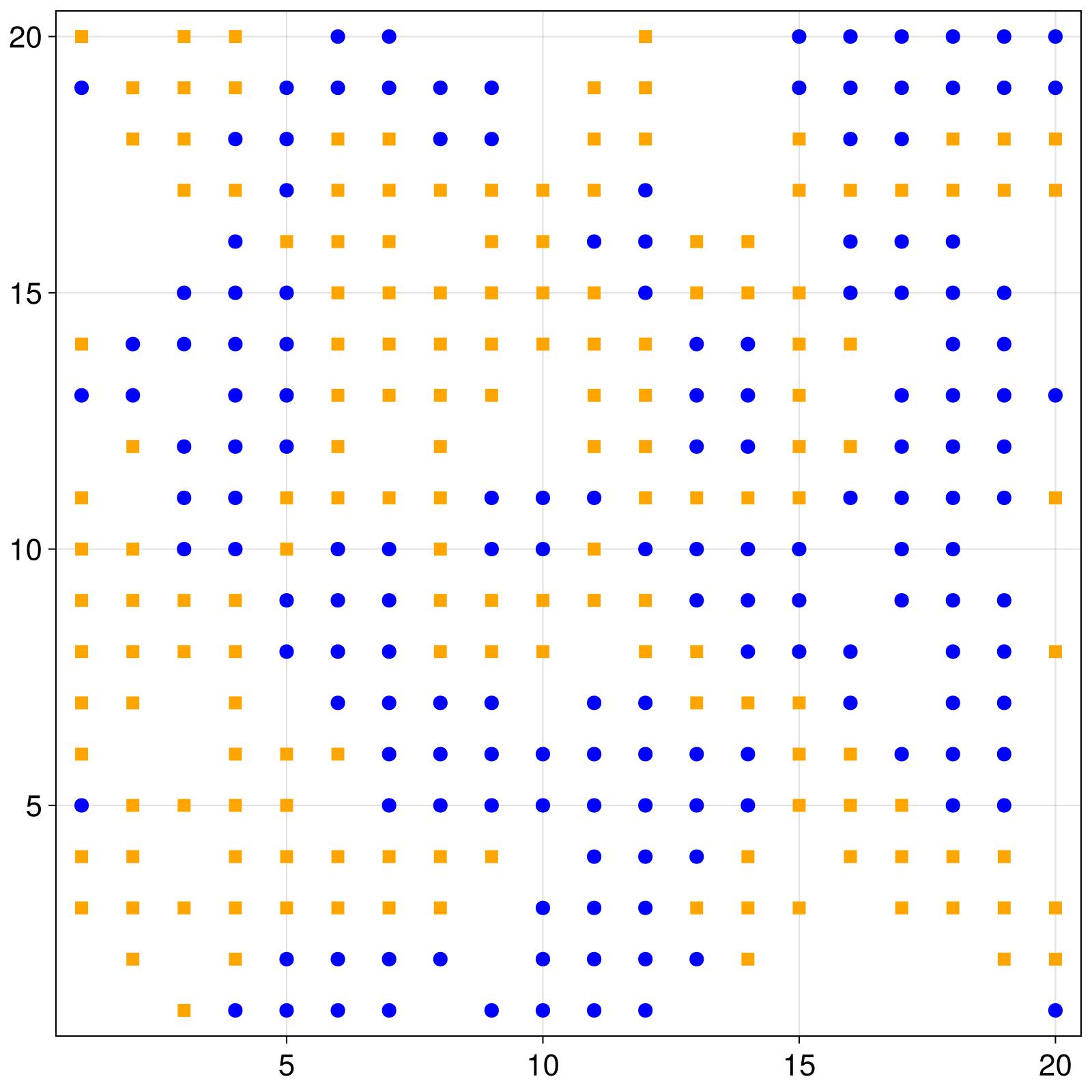

The function abmvideo can be used to save an animation of the ABM into a video.

schelling = initialize()
abmvideo(
    "schelling.mp4", schelling;
    agent_color = groupcolor, agent_marker = groupmarker, as = 10,
    framerate = 4, frames = 20,
    title = "Schelling's segregation model"
)

┌ Warning: Keywords `as, am, ac` has been deprecated in favor of
│           `agent_size, agent_marker, agent_color`
└ @ AgentsVisualizations ~/work/Agents.jl/Agents.jl/ext/AgentsVisualizations/src/abmplot.jl:70

Step 7: data collection

Running the model and collecting data while the model runs is done with the run! function. Besides run!, there is also the paramscan function that performs data collection while scanning ranges of the parameters of the model, and the ensemblerun! that performs ensemble simulations and data collection.

The run! function has been designed for maximum flexibility: practically all scenarios of data collection are possible, whether you need agent data, model data, aggregated data, or arbitrary combinations.

To use run! we simply provide a vector of what agent properties to collect as data. The adata keyword corresponds to the "agent data", and there is the mdata keyword for model data.

For example, specifying the properties as Symbols means to collect the named properties

adata = [:pos, :mood, :group]

schelling = initialize()
adf, mdf = run!(schelling, 5; adata) # run for 5 steps
adf[end-10:end, :] # display only the last few rows

run! collects data in the form of a DataFrame which is Julia's premier format for tabular data (and you probably need to learn how to use it independently of Agents.jl if you don't know it yet, see the documentation of DataFrames.jl to do so). Above, data were collected for each agent and for each step of the simulation.

Besides Symbols, we can specify functions as agent data to collect

x(agent) = agent.pos[1]
schelling = initialize()
adata = [x, :mood, :group]
adf, mdf = run!(schelling, 5; adata)
adf[end-10:end, :] # display only the last few rows

With the above adata vector, we collected all agent's data. We can instead collect aggregated data for the agents. For example, let's only get the number of happy individuals, and the average of the "x" (not very interesting, but anyway!). To do this, make adata a vector of Tuples, where the first entry of the tuple is the data to collect, and the second how to aggregate it over agents.

using Statistics: mean
schelling = initialize();
adata = [(:mood, sum), (x, mean)]
adf, mdf = run!(schelling, 5; adata)
adf

Other examples in the documentation are more realistic, with more meaningful collected data. You should consult the documentation of run! for more power over data collection.

And this concludes the main tutorial!

Multiple agent types in Agents.jl

In realistic modelling situations it is often the case the the ABM is composed of different types of agents. Agents.jl supports two approaches for multi-agent ABMs. The first uses the Union type (this subsection), and the second uses the @multiagent command (next subsection). @multiagent is recommended as default, because in many cases it will have performance advantages over the Union approach without having tangible disadvantages. However, we strongly recommend you to read through the comparison of the two approaches.

Note that using multiple agent types is a possibility entirely orthogonal to the type of AgentBasedModel or the type of space. Everything we describe here works for any Agents.jl simulation.

Multiple agent types with Union types

The simplest way to add more agent types is to make more of them with @agent and then give a Union of agent types as the agent type when making the AgentBasedModel. For example, let's say that a new type of agent enters the simulation; a politician that would "attract" a preferred demographic. We then would make

@agent struct Politician(GridAgent{2})
    preferred_demographic::Int
end

and, when making the model we would specify

model = StandardABM(
    Union{SchellingAgent, Politician}, # type of agents
    space; # space they live in
)

StandardABM with 0 agents of type Union{Main.Politician, Main.SchellingAgent}
 agents container: Dict
 space: GridSpaceSingle with size (10, 10), metric=chebyshev, periodic=false
 scheduler: fastest

Naturally, we would have to define a new agent stepping function that would act differently depending on the agent type. This could be done by making a function that calls other functions depending on the type, such as

function union_step!(agent, model)
    if typeof(agent) <: AgentSchelling
        schelling_step!(agent, model)
    elseif typeof(agent) <: Politician
        politician_step!(agent, model)
    end
end

union_step! (generic function with 1 method)

and then passing

model = StandardABM(
    Union{SchellingAgent, Politician}, # type of agents
    space; # space they live in
    agent_step! = union_step!
)

StandardABM with 0 agents of type Union{Main.Politician, Main.SchellingAgent}
 agents container: Dict
 space: GridSpaceSingle with size (10, 10), metric=chebyshev, periodic=false
 scheduler: fastest

This approach also works with the @multiagent possibility we discuss below. Union types however also offer the unique possibility of utilizing Julia's multiple dispatch system. Hence, we can use the same function name and add dispatch to it, such as:

function dispatch_step!(agent::SchellingAgent, model)
    # stuff.
end

function dispatch_step!(agent::Politician, model)
    # other stuff.
end

dispatch_step! (generic function with 2 methods)

and give dispatch_step! to the agent_step! keyword during model creation.

Multiple agent types with @multiagent

@multiagent does not offer the multiple dispatch possibility, but in the majority of cases leads to better computational performance. Intentionally the command has been designed to be as similar to @agent as possible. The syntax to use it is like so:

@multiagent struct MultiSchelling{X}(GridAgent{2})
    @subagent struct Civilian # can't re-define existing `Schelling` name
        mood::Bool = false
        group::Int
    end
    @subagent struct Governor{X} # can't redefine existing `Politician` name
        group::Int
        influence::X
    end
end

This macro created three names into scope:

(MultiSchelling, Civilian, Governor)

(Main.MultiSchelling, Main.Civilian, Main.Governor)

however, only one of these names is an actual Julia type:

fieldnames(MultiSchelling)

(:id, :pos, :mood, :group, :influence, Symbol("##_kind#823"))

that contains all fields of all subtypes without duplication, while

fieldnames(Civilian)

()

doesn't have any fields. Instead, you should think of Civilian and Governor as just convenience functions that have been defined for you to "behave like" types. E.g., you can initialize

civ = Civilian(; id = 2, pos = (2, 2), group = 2) # default `mood`

Civilian(2, (2, 2), false, 2)::Main.MultiSchelling

or

gov = Governor(; id = 3 , pos = (2, 2), group = 2, influence = 0.5)

Governor{Float64}(3, (2, 2), 2, 0.5)::Main.MultiSchelling

exactly as if these were types made with @agent. These are all of type MultiSchelling

typeof(gov)

Main.MultiSchelling{Float64}

and hence you can't use typeof to differentiate them. But you can use

kindof(gov)

:Governor

instead. Hence, the agent stepping function should be something like

function multi_step!(agent, model)
    if kindof(agent) == :Civilian
        schelling_step!(agent, model)
    elseif kindof(agent) == :Governor
        politician_step!(agent, model)
    end
end

multi_step! (generic function with 1 method)

and give that to the model creation

model = StandardABM(
    MultiSchelling, # the multi-agent supertype is given as the type
    space;
    agent_step! = multi_step!
)

StandardABM with 0 agents of type Main.MultiSchelling
 agents container: Dict
 space: GridSpaceSingle with size (10, 10), metric=chebyshev, periodic=false
 scheduler: fastest

Adding agents of different types to the model

Regardless of whether you went down the Union or @multiagent route, the API of Agents.jl has been designed such that there is no difference in subsequent usage. To add agents to a model, we use the existing add_agent_single! command, but now specifying as a first argument the type of agent to add.

For example, in the union case we provide the Union type when we create the model,

model = StandardABM(Union{SchellingAgent, Politician}, space)

StandardABM with 0 agents of type Union{Main.Politician, Main.SchellingAgent}
 agents container: Dict
 space: GridSpaceSingle with size (10, 10), metric=chebyshev, periodic=false
 scheduler: fastest

we add them by specifying the type

add_agent_single!(SchellingAgent, model; group = 1, mood = true)

Main.SchellingAgent(1, (3, 7), true, 1)

or

add_agent_single!(Politician, model; preferred_demographic = 1)

Main.Politician(2, (8, 7), 1)

and we see

collect(allagents(model))

2-element Vector{Union{Main.Politician, Main.SchellingAgent}}:
 Main.Politician(2, (8, 7), 1)
 Main.SchellingAgent(1, (3, 7), true, 1)

For the @multiagent case, there is really no difference. We have

model = StandardABM(MultiSchelling, space)

StandardABM with 0 agents of type Main.MultiSchelling
 agents container: Dict
 space: GridSpaceSingle with size (10, 10), metric=chebyshev, periodic=false
 scheduler: fastest

we add

add_agent_single!(Civilian, model; group = 1)

Civilian(1, (8, 3), false, 1)::Main.MultiSchelling

or

add_agent_single!(Governor, model; influence = 0.5, group = 1)

Governor{Float64}(2, (6, 1), 1, 0.5)::Main.MultiSchelling

and we see

collect(allagents(model))

2-element Vector{Main.MultiSchelling}:
 Governor{Float64}(2, (6, 1), 1, 0.5)::Main.MultiSchelling
 Civilian(1, (8, 3), false, 1)::Main.MultiSchelling

And that's the end of the tutorial!!! You can visit other examples to see other types of usage of Agents.jl, or go into the API to find the functions you need to make your own ABM!