Detecting & Categorizing Chaos
Being able to detect and distinguish chaotic from regular behavior is crucial in the study of dynamical systems. Most of the time a positive maximum lyapunov exponent and a bounded system indicate chaos.
However, the convergence of the Lyapunov exponent can be slow, or even misleading, as the types of chaotic behavior vary with respect to their predictability. There are some alternatives, some more efficient and some more accurate in characterizing chaotic and regular motion.
Generalized Alignment Index
"GALI" for short, is a method that relies on the fact that initially orthogonal deviation vectors tend to align towards the direction of the maximum Lyapunov exponent for chaotic motion. It is one of the most recent and cheapest methods for distinguishing chaotic and regular behavior, introduced first in 2007 by Skokos, Bountis & Antonopoulos.
ChaosTools.gali — Function
gali(ds::DynamicalSystem, T, k::Int; kwargs...) -> GALI_k, tCompute $\text{GALI}_k$[Skokos2007] for a given k up to time T. Return $\text{GALI}_k(t)$ and time vector $t$.
The third argument sets the order of gali. gali function simply initializes a TangentDynamicalSystem with k deviation vectors and calls the method below. This means that the automatic Jacobian is used by default. Initialize manually a TangentDynamicalSystem if you have a hand-coded Jacobian.
Keyword arguments
threshold = 1e-12: IfGALI_kfalls below thethresholditeration is terminated.Δt = 1: Time-step between deviation vector normalizations. For continuous systems this is approximate.u0: Initial state for the system. Defaults tocurrent_state(ds).
Description
The Generalized Alignment Index, $\text{GALI}_k$, is an efficient (and very fast) indicator of chaotic or regular behavior type in $D$-dimensional Hamiltonian systems ($D$ is number of variables). The asymptotic behavior of $\text{GALI}_k(t)$ depends critically on the type of orbit resulting from the initial condition. If it is a chaotic orbit, then
\[\text{GALI}_k(t) \sim \exp\left[\sum_{j=1}^k (\lambda_1 - \lambda_j)t \right]\]
with $\lambda_j$ being the j-th Lyapunov exponent (see lyapunov, lyapunovspectrum). If on the other hand the orbit is regular, corresponding to movement in $d$-dimensional torus with $1 \le d \le D/2$ then it holds
\[\text{GALI}_k(t) \sim \begin{cases} \text{const.}, & \text{if} \;\; 2 \le k \le d \; \; \text{and} \; \;d > 1 \\ t^{-(k - d)}, & \text{if} \;\; d < k \le D - d \\ t^{-(2k - D)}, & \text{if} \;\; D - d < k \le D \end{cases}\]
Traditionally, if $\text{GALI}_k(t)$ does not become less than the threshold until T the given orbit is said to be chaotic, otherwise it is regular.
Our implementation is not based on the original paper, but rather in the method described in[Skokos2016b], which uses the product of the singular values of $A$, a matrix that has as columns the deviation vectors.
gali(tands::TangentDynamicalSystem, T; threshold = 1e-12, Δt = 1)The low-level method that is called by gali(ds::DynamicalSystem, ...). Use this method for looping over different initial conditions or parameters by calling reinit! to tands.
The order of $\text{GALI}_k$ computed is the amount of deviation vectors in tands.
Also use this method if you have a hand-coded Jacobian to pass when creating tands.
GALI example
As an example let's use the Henon-Heiles system
using ChaosTools, CairoMakie
using OrdinaryDiffEq: Vern9

function henonheiles_rule(u, p, t)
    SVector(u[3], u[4],
        -u[1] - 2u[1]*u[2],
        -u[2] - (u[1]^2 - u[2]^2),
    )
end
function henonheiles_jacob(u, p, t)
    SMatrix{4,4}(0, 0, -1 - 2u[2], -2u[1], 0, 0,
     -2u[1], -1 + 2u[2], 1, 0, 0, 0, 0, 1, 0, 0)
end

u0=[0, -0.25, 0.42081, 0]
Δt = 1.0
diffeq = (abstol=1e-9, retol=1e-9, alg = Vern9(), maxiters = typemax(Int))
sp = [0, .295456, .407308431, 0] # stable periodic orbit: 1D torus
qp = [0, .483000, .278980390, 0] # quasiperiodic orbit: 2D torus
ch = [0, -0.25, 0.42081, 0]      # chaotic orbit
ds = CoupledODEs(henonheiles_rule, sp)
4-dimensional CoupledODEs
deterministic: true
discrete time: false
in-place: false
dynamic rule: henonheiles_rule
ODE solver: Tsit5
ODE kwargs: (abstol = 1.0e-6, reltol = 1.0e-6)
parameters: SciMLBase.NullParameters()
time: 0.0
state: [0.0, 0.295456, 0.407308431, 0.0]
Let's see what happens with a quasi-periodic orbit:
tr = trajectory(ds, 10000.0, qp; Δt)[1]
fig, ax = scatter(tr[:,1], tr[:,3]; label="qp", markersize=2)
axislegend(ax)

ax = Axis(fig[1,2]; yscale = log)
for k in [2,3,4]
    g, t = gali(ds, 10000.0, k; u0 = qp, Δt)
    logt = log.(t)
    lines!(ax, logt, g; label="GALI_$(k)")
    if k == 2
        lines!(ax, logt, 1 ./ t.^(2k-4); label="slope -$(2k-4)")
    else
        lines!(ax, logt, 100 ./ t.^(2k-4); label="slope -$(2k-4)")
    end
end
ylims!(ax, 1e-12, 2)
fig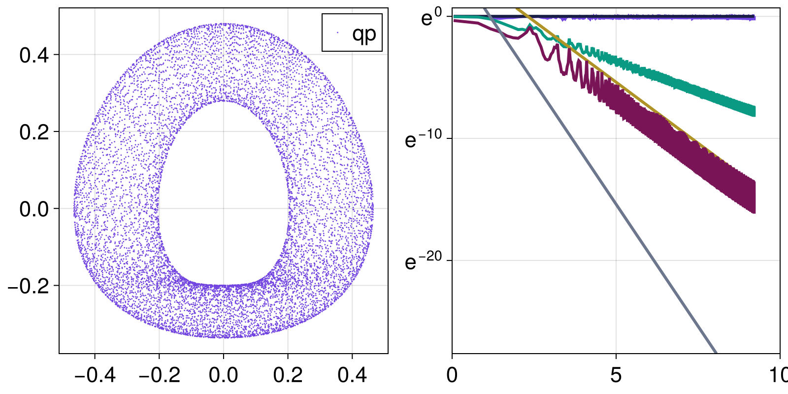
And here is GALI of a continuous system with a chaotic orbit
tr = trajectory(ds, 10000.0, ch; Δt)[1]
fig, ax = scatter(tr[:,1], tr[:,3]; label="ch", markersize=2, color = (Main.COLORS[1], 0.5))
axislegend(ax)

ax = Axis(fig[1,2]; yscale = log)
ls = lyapunovspectrum(ds, 5000; Δt, u0 = ch)
for k in [2,3,4]
    ex = sum(ls[1] - ls[j] for j in 2:k)
    g, t = gali(ds, 1000, k; u0 = ch, Δt)
    lines!(t, exp.(-ex.*t); label="exp. k=$k")
    lines!(t, g; label="GALI_$(k)")
end
ylims!(ax, 1e-16, 1)
fig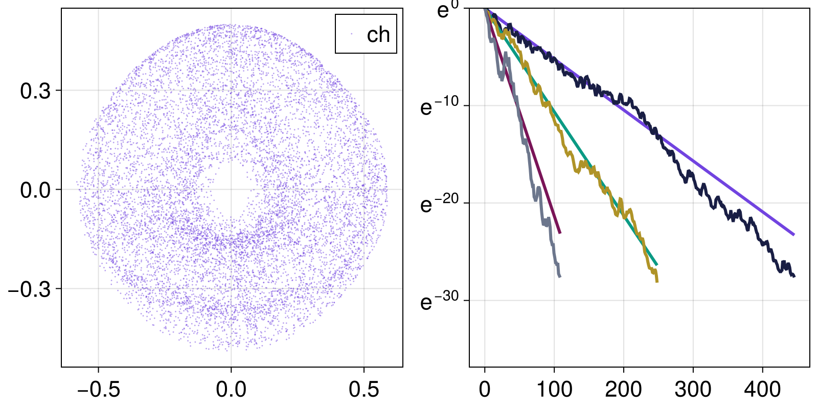
Using GALI
No-one in their right mind would try to fit power-laws in order to distinguish between chaotic and regular behavior, like the above examples. These were just proofs that the method works as expected.
The most common usage of $\text{GALI}_k$ is to define a (sufficiently) small amount of time and a (sufficiently) small threshold and see whether $\text{GALI}_k$ stays below it, for a (sufficiently) big $k$.
For example, we utilize parallel integration of TangentDynamicalSystem to compute $GALI$ for many initial conditions and produce a color-coded map of regular and chaotic orbits of the standard map.
The following is an example of advanced usage:
using ChaosTools, CairoMakie
# Initialize `TangentDynamicalSystem`
@inbounds function standardmap_rule(x, par, n)
    theta = x[1]; p = x[2]
    p += par[1]*sin(theta)
    theta += p
    return mod2pi.(SVector(theta, p))
end
@inbounds standardmap_jacob(x, p, n) = SMatrix{2,2}(
    1 + p[1]*cos(x[1]), p[1]*cos(x[1]), 1, 1
)
ds = DeterministicIteratedMap(standardmap_rule, ones(2), [1.0])
tands = TangentDynamicalSystem(ds; J = standardmap_jacob)
# Collect initial conditions
dens = 101
θs = ps = range(0, stop = 2π, length = dens)
ics = vec(SVector{2, Float64}.(Iterators.product(θs, ps)))
# Perform loop
regularity = zeros(size(ics))
for i in eachindex(ics)
    u0 = ics[i]
    reinit!(ds, u0)
    regularity[i] = gali(ds, 500)[2][end]
end
# Visualize
fig, ax, sc = scatter(ics; color = regularity)
Colorbar(fig[1,2], sc; label = "regularity")
fig
You can parallelize this code as well, see the main tutorial of DynamicalSystems.jl for an example.
Predictability of a chaotic system
Even if a system is "formally" chaotic, it can still be in phases where it is partially predictable, because the correlation coefficient between nearby trajectories vanishes very slowly with time. Wernecke, Sándor & Gros have developed an algorithm that allows one to classify a dynamical system to one of three categories: strongly chaotic, partially predictable chaos or regular (called laminar in their paper).
We have implemented their algorithm in the function predictability. Note that we set up the implementation to always return regular behavior for negative Lyapunov exponent. You may want to override this for research purposes.
ChaosTools.predictability — Function
predictability(ds::CoreDynamicalSystem; kwargs...) -> chaos_type, ν, CDetermine whether ds displays strongly chaotic, partially-predictable chaotic or regular behaviour, using the method by Wernecke et al. described in[Wernecke2017].
Return the type of the behavior, the cross-distance scaling coefficient ν and the correlation coefficient C. Typical values for ν, C and chaos_type are given in Table 2 of[Wernecke2017]:
chaos_type | ν | C |
|---|---|---|
:SC | 0 | 0 |
:PPC | 0 | 1 |
:REG | 1 | 1 |
If none of these conditions apply, the return value is :IND (for indeterminate).
Keyword arguments
Ttr = 200: Extra transient time to evolve the system before sampling from the trajectory. Should beIntfor discrete systems.T_sample = 1e4: Time to evolve the system for taking samples. Should beIntfor discrete systems.n_samples = 500: Number of samples to take for use in calculating statistics.λ_max = lyapunov(ds, 5000): Value to use for largest Lyapunov exponent for finding the Lyapunov prediction time. If it is less than zero a regular result is returned immediately.d_tol = 1e-3: tolerance distance to use for calculating Lyapunov prediction time.T_multiplier = 10: Multiplier from the Lyapunov prediction time to the evaluation time.T_max = Inf: Maximum time at which to evaluate trajectory distance. If the internally computed evaluation time is larger thanT_max, stop atT_maxinstead. It is strongly recommended to manually set this!δ_range = 10.0 .^ (-9:-6): Range of initial condition perturbation distances to use to determine scalingν.ν_threshold = C_threshold = 0.5: Thresholds for scaling coefficients (they become 0 or 1 if they are less or more than the threshold).
Description
The algorithm samples points from a trajectory of the system to be used as initial conditions. Each of these initial conditions is randomly perturbed by a distance δ, and the trajectories for both the original and perturbed initial conditions are evolved up to the 'evaluation time' T (see below its definition).
The average (over the samples) distance and cross-correlation coefficient of the state at time T is computed. This is repeated for a range of δ (defined by δ_range), and linear regression is used to determine how the distance and cross-correlation scale with δ, allowing for identification of chaos type.
The evaluation time T is calculated as T = T_multiplier*Tλ, where the Lyapunov prediction time Tλ = log(d_tol/δ)/λ_max. This may be very large if the λ_max is small, e.g. when the system is regular, so this internally computed time T can be overridden by a smaller T_max set by the user.
Performance Notes
For continuous systems, it is likely that the maxiters used by the integrators needs to be increased, e.g. to 1e9. This is part of the diffeq kwargs. In addition, be aware that this function does a lot of internal computations. It is operating in a different speed than e.g. lyapunov.
Example Hénon Map
We will create something similar to figure 2 of the paper, but for the Hénon map.
fig = Figure()
ax = Axis(fig[1,1]; xlabel = L"a", ylabel = L"x")
henon_rule(x, p, n) = SVector{2}(1.0 - p[1]*x[1]^2 + x[2], p[2]*x[1])
he = DeterministicIteratedMap(henon_rule, zeros(2), [1.4, 0.3])
as = 0.8:0.01:1.225
od = orbitdiagram(he, 1, 1, as; n = 2000, Ttr = 2000)
colors = Dict(:REG => "blue", :PPC => "green", :SC => "red")
for (i, a) in enumerate(as)
    set_parameter!(he, 1, a)
    chaos_type, ν, C = predictability(he; T_max = 400000, Ttr = 2000)
    scatter!(ax, a .* ones(length(od[i])), od[i];
    color = (colors[chaos_type], 0.05), markersize = 2)
end
ax.title = "predictability of Hénon map"
fig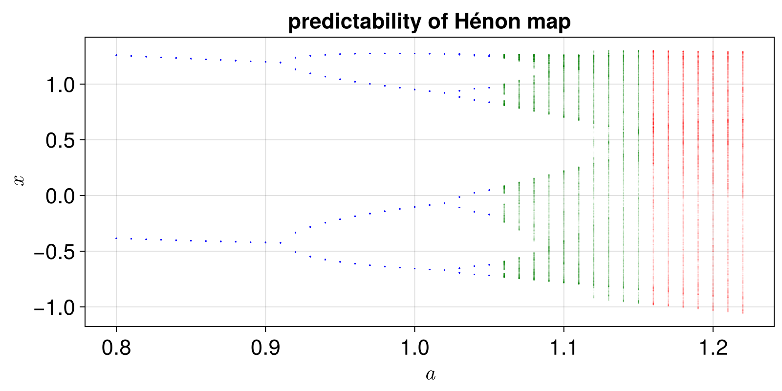
The 0-1 test for chaos
The methods mentioned in this page so far require a DynamicalSystem instance. But of course this is not always the case. The so-called "0 to 1" test for chaos, by Gottwald & Melbourne, takes as an input a timeseries and outputs a boolean true if the timeseries is chaotic or false if it is not.
Notice that the method does have a lot of caveats, so you should read the review paper before using. Also, it doesn't work for noisy data.
ChaosTools.testchaos01 — Function
testchaos01(x::Vector [, cs, N0]) -> chaotic?Perform the so called "0-1" test for chaos introduced by Gottwald and Melbourne[Gottwald2016] on the timeseries x. Return true if x is chaotic, false otherwise.
Description
This method tests if the given timeseries is chaotic or not by transforming it into a two-dimensional diffusive process like so:
\[p_n = \sum_{j=1}^{n}\phi_j \cos(j c),\quad q_n = \sum_{j=1}^{n}\phi_j \sin(j c)\]
If the timeseries is chaotic, the mean square displacement of the process grows as sqrt(length(x)), while it stays constant if the timeseries is regular.
The implementation here computes K, a coefficient measuring the growth of the mean square displacement, and simply checks if K > 0.5. K is the median of $K_c$ over given c, see the reference.
If you want to access the various Kc you should call the method testchaos01(x, c::Real, N0) which returns Kc. In fact, the high level method is just median(testchaos01(x, c, N0) for c in cs) > 0.5.
cs defaults to 3π/5*rand(100) + π/4 and N0, the length of the two-dimensional process, is N0 = length(x)/10.
For data sampled from continuous dynamical systems, some care must be taken regarding the values of cs. Also note that this method performs rather poorly with even the slight amount of noise, returning true for even small amounts of noise noisy timeseries. Some possibilities to alleviate this exist, but are context specific on the application. See [Gottwald2016] for more info.
Expansion entropy
The expansion entropy is a quantity that is suggested by B. Hunt and E. Ott as a measure that can define chaos (so far no widely accepted definition of chaos exists). Positive expansion entropy means chaos.
ChaosTools.expansionentropy — Function
expansionentropy(ds::DynamicalSystem, sampler, isinside; kwargs...)Calculate the expansion entropy[Hunt2015] of ds, in the restraining region $S$ by estimating the slope (via linear regression) of the curve $\log E_{t0+T, t0}(f, S)$ versus $T$ (using linear_region). This is an approximation of the expansion entropy $H_0$, according to[Hunt2015]. Return $T$, $\log E$ and the calculated slope.
sampler is a 0-argument function that generates a random initial conditions of ds and isinside is a 1-argument function that given a state it returns true if the state is inside the restraining region. Typically sampler, isinside are the output of statespace_sampler.
Keyword arguments
N = 1000: Number of samples taken at each batch (same as $N$ of [Hunt2015]).steps = 40: The maximal steps for which the system will be run.batches = 100: Number of batches to run the calculation, see below.Δt = 1: Time evolution step size.J = nothing: Jacobian function given toTangentDynamicalSystem.
Description
N samples are initialized and propagated forwards in time (along with their tangent space). At every time $t$ in [t0+Δt, t0+2Δt, ..., t0+steps*Δt] we calculate $H$:
\[H[t] = \log E_{t0+T, t0}(f, S),\]
with
\[E_{t0+T, t0}(f, S) = \frac 1 N \sum_{i'} G(Df_{t0+t, t0}(x_i))\]
(using same notation as [Hunt2015]). In principle $E$ is the average largest possible growth ratio within the restraining region (sampled by the initial conditions). The summation is only over $x_i$ that stay inside the region $S$ defined by the boolean function isinside. This process is done by the ChaosTools.expansionentropy_sample function.
Then, this is repeated for batches amount of times, as recommended in[Hunt2015]. From all these batches, the mean and std of $H$ is computed at every time point. This is done by the expansionentropy_batch function. When plotted versus $t$, these create the curves and error bars of e.g. Figs 2, 3 of [1].
This function expansionentropy simply returns the slope of the biggest linear region of the curve $H$ versus $t$, which approximates the expansion entropy $H_0$. It is therefore recommended to use expansionentropy_batch directly and evaluate the result yourself, as this step is known to be inaccurate for non-chaotic systems (where $H$ fluctuates strongly around 0).
- Skokos2007Skokos, C. H. et al., Physica D 231, pp 30–54 (2007)
- Skokos2016bSkokos, C. H. et al., Chaos Detection and Predictability - Chapter 5 (section 5.3.1 and ref. [85] therein), Lecture Notes in Physics 915, Springer (2016)
- Wernecke2017Wernecke, H., Sándor, B. & Gros, C. How to test for partially predictable chaos. Scientific Reports 7, (2017).
- Gottwald2016Gottwald & Melbourne, “The 0-1 test for chaos: A review” Lect. Notes Phys., vol. 915, pp. 221–247, 2016.
- Hunt2015Hunt & Ott, ‘Defining Chaos’, Chaos 25.9 (2015)