Orbit diagrams

An orbit diagram is a way to visualize the asymptotic behaviour of a map, when a parameter of the system is changed. In practice an orbit diagram is a simple plot that plots the last n states of a dynamical system at a given parameter, repeated for all parameters in a range of interest. While this concept can apply to any kind of system, it makes most sense in discrete time dynamical systems. See Chapter 4 of Nonlinear Dynamics, Datseris & Parlitz, Springer 2022, for a more involved discussion on orbit diagrams for both discrete and continuous time systems.

ChaosTools.orbitdiagram — Function

orbitdiagram(ds::DynamicalSystem, i, p_index, pvalues; kwargs...) → od

Compute the orbit diagram (sometimes wrongly called bifurcation diagram) of the given dynamical system, saving the i variable(s) for parameter values pvalues. The p_index specifies which parameter to change via set_parameter!(ds, p_index, pvalue). Works for any kind of DynamicalSystem, although it mostly makes sense with one of DeterministicIteratedMap, StroboscopicMap, PoincareMap.

An orbit diagram is simply a collection of the last n states of ds as ds is evolved. This is done for each parameter value.

i can be Int or AbstractVector{Int}. If i is Int, od is a vector of vectors. Else od is a vector of vectors of vectors. Each entry od od are the points at each parameter value, so that length(od) == length(pvalues) and length(od[j]) == n, ∀ j.

Keyword arguments

n::Int = 100: Amount of points to save for each parameter value.
Δt = 1: Stepping time between saving points.
u0 = nothing: Specify an initial state. If nothing, the previous state after each parameter is used to seed the new initial condition at the new parameter (with the very first state being the system's state). This makes convergence to the attractor faster, necessitating smaller Ttr. Otherwise u0 can be a standard state, or a vector of states, so that a specific state is used for each parameter.
Ttr::Int = 10: Each orbit is evolved for Ttr first before saving output.
ulims = (-Inf, Inf): only record system states within ulims (only valid if i isa Int). Iteration continues until n states fall within ulims.
show_progress = false: Display a progress bar (counting the parameter values).
periods = nothing: Only valid if ds isa StroboscopicMap. If given, it must be a a container with same layout as pvalues. Provides a value for the period for each parameter value. Useful in case the orbit diagram is produced versus a driving frequency.

source

Deterministic iterated map

For example, let's compute the famous orbit diagram of the logistic map:

using ChaosTools, CairoMakie

logistic_rule(x, p, n) = @inbounds SVector(p[1]*x[1]*(1-x[1]))
logistic = DeterministicIteratedMap(logistic_rule, [0.4], [4.0])

i = 1
parameter = 1
pvalues = 2.5:0.004:4
n = 2000
Ttr = 2000
output = orbitdiagram(logistic, i, parameter, pvalues; n, Ttr)

L = length(pvalues)
x = Vector{Float64}(undef, n*L)
y = copy(x)
for j in 1:L
    x[(1 + (j-1)*n):j*n] .= pvalues[j]
    y[(1 + (j-1)*n):j*n] .= output[j]
end

fig, ax = scatter(x, y; axis = (xlabel = L"r", ylabel = L"x"),
    markersize = 0.8, color = ("black", 0.05),
)
ax.title = "Logistic map orbit diagram"
xlims!(ax, pvalues[1], pvalues[end]); ylims!(ax,0,1)
fig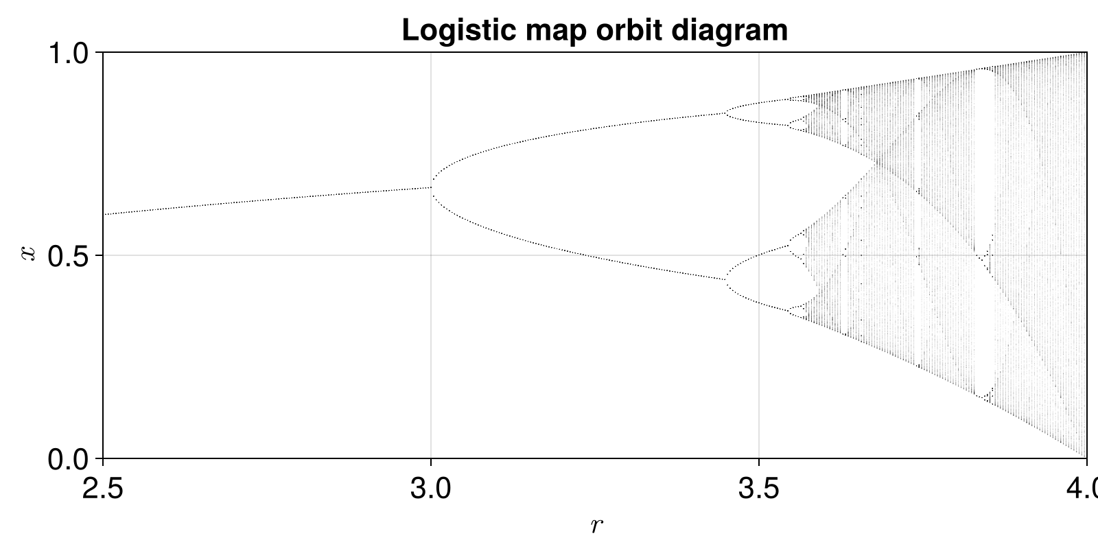

Stroboscopic map

The beauty of orbitdiagram is that it can be directly applied to any kind of DynamicalSystem. The most useful cases are the already seen DeterministicIteratedMap, but also PoincareMap and StroboscopicMap. Here is an example of the orbit diagram for the Duffing oscillator (making the same as Figure 9.2 of Nonlinear Dynamics, Datseris & Parlitz, Springer 2022).

using ChaosTools, CairoMakie

function duffing_rule(u,p,t)
    d, a, ω = p
    du1 =  u[2]
    du2 =  -u[1] - u[1]*u[1]*u[1] - d*u[2] + a*sin(ω*t)
    return SVector(du1, du2)
end
T0 = 25.0
p0 = [0.1, 7, 2π/T0]
u0 = [1.1, 1.1]
ds = CoupledODEs(duffing_rule, u0, p0)
duffing = StroboscopicMap(ds, T0)

# We want to change both the parameter `ω`, but also the
# period of the stroboscopic map. `orbitdiagram` allows this!
Trange = range(8, 26; length = 201)
ωrange = @. 2π / Trange
n = 200
output = orbitdiagram(duffing, 1, 3, ωrange; n, u0, Ttr = 100, periods = Trange)

L = length(Trange)
x = Vector{Float64}(undef, n*L)
y = copy(x)
for j in 1:L
    x[(1 + (j-1)*n):j*n] .= Trange[j]
    y[(1 + (j-1)*n):j*n] .= output[j]
end

fig, ax = scatter(x, y; axis = (xlabel = L"T", ylabel = L"u_1"),
    markersize = 8, color = ("blue", 0.25),
)
ylims!(ax, -1, 1)
fig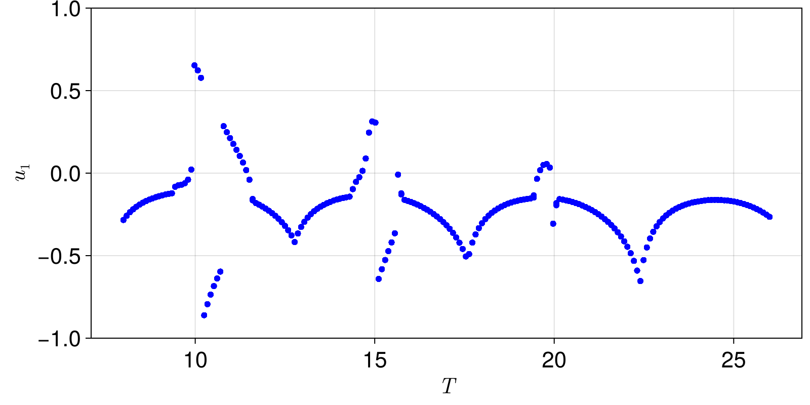

Pro tip: to actually make Fig. 9.2 you'd have to do two modifications: first, pass periods = Trange ./ 2, so that points are recorded every half period. Then, at the very end, do y[2:2:end] .= -y[2:2:end] so that the symmetric orbits are recorded as well