Dimensionality reduction

Broomhead-King Coordinates

ChaosTools.broomhead_king — Function

broomhead_king(s::AbstractVector, d::Int) -> U, S, Vtr

Return the Broomhead-King coordinates of a timeseries s by performing svd on high-dimensional delay embedding if s with dimension d with minimum delay.

Description

Broomhead and King coordinates is an approach proposed in ^{[Broomhead1987]} that applies the Karhunen–Loève theorem to delay coordinates embedding with smallest possible delay.

The function performs singular value decomposition on the d-dimensional matrix $X$ of $s$,

\[X = \frac{1}{\sqrt{N}}\left( \begin{array}{cccc} x_1 & x_2 & \ldots & x_d \\ x_2 & x_3 & \ldots & x_{d+1}\\ \vdots & \vdots & \vdots & \vdots \\ x_{N-d+1} & x_{N-d+2} &\ldots & x_N \end{array} \right) = U\cdot S \cdot V^{tr}.\]

where $x := s - \bar{s}$. The columns of $U$ can then be used as a new coordinate system, and by considering the values of the singular values $S$ you can decide how many columns of $U$ are "important".

source

This alternative/improvement of the traditional delay coordinates can be a very powerful tool. An example where it shines is noisy data where there is the effect of superficial dimensions due to noise.

Take the following example where we produce noisy data from a system and then use Broomhead-King coordinates as an alternative to "vanilla" delay coordinates:

using ChaosTools, CairoMakie

function gissinger_rule(u, p, t)
    μ, ν, Γ = p
    du1 = μ*u[1] - u[2]*u[3]
    du2 = -ν*u[2] + u[1]*u[3]
    du3 = Γ - u[3] + u[1]*u[2]
    return SVector{3}(du1, du2, du3)
end

gissinger = CoupledODEs(gissinger_rule, ones(3), [0.112, 0.1, 0.9])
X, t = trajectory(gissinger, 1000.0; Ttr = 100, Δt = 0.1)
x = X[:, 1]

L = length(x)
s = x .+ 0.5rand(L) #add noise

U, S = broomhead_king(s, 20)
summary(U)

"9982×20 Matrix{Float64}"

Now let's simply compare the above result with the one you get from doing a standard delay coordinates embedding

using DelayEmbeddings: embed, estimate_delay

fig = Figure()
axs = [Axis3(fig[1, i]) for i in 1:2]
lines!(axs[1], U[:, 1], U[:, 2], U[:, 3])
axs[1].title = "Broomhead-King of s"

R = embed(s, 3, estimate_delay(x, "mi_min"))
lines!(axs[2], columns(R)...)
axs[2].title = "2D embedding of s"
fig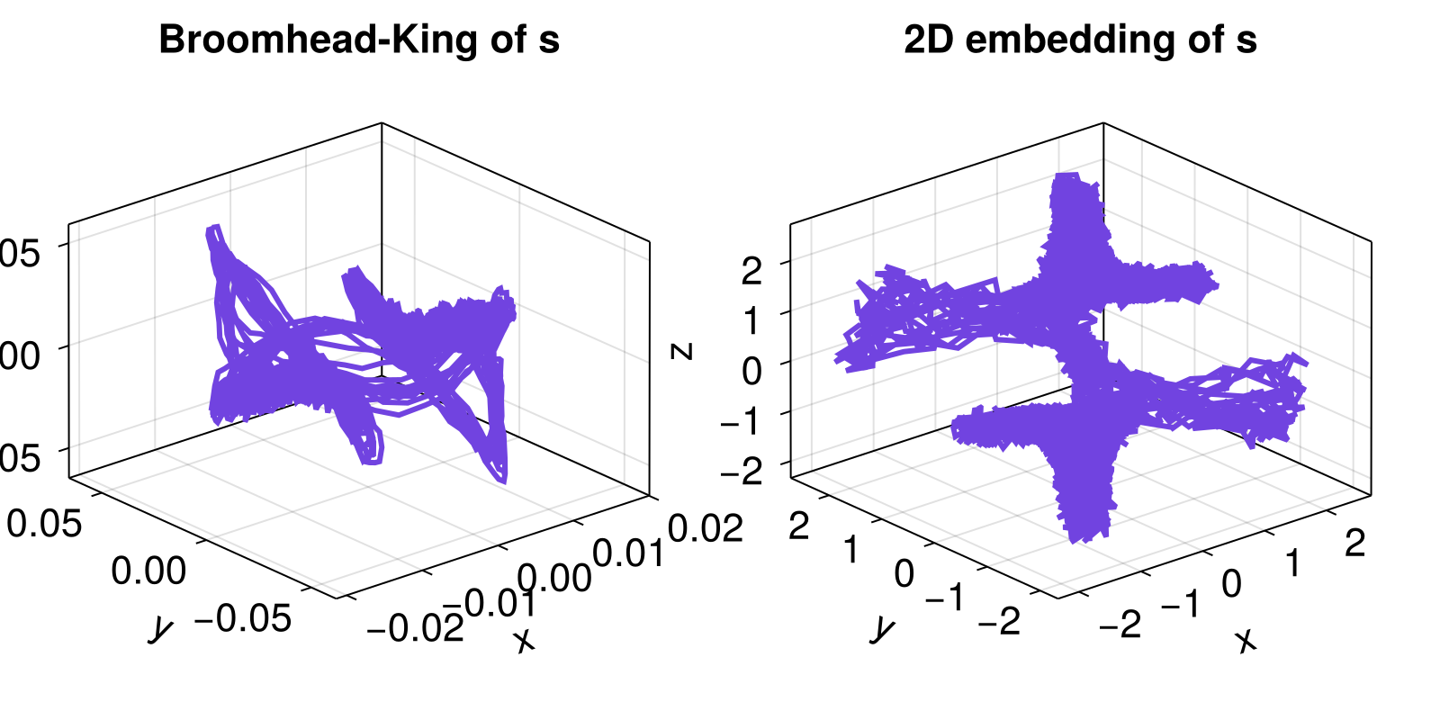

we have used the same system as in the Delay Coordinates Embedding example, and picked the optimal delay time of τ = 30 (for same Δt = 0.05). Regardless, the vanilla delay coordinates is much worse than the Broomhead-King coordinates.

DyCA - Dynamical Component Analysis

ChaosTools.dyca — Function

dyca(data, eig_threshold) -> eigenvalues, proj_mat, projected_data

Compute the Dynamical Component analysis (DyCA) of the given data^[Uhl2018] used for dimensionality reduction.

Return the eigenvalues, projection matrix, and reduced-dimension data (which are just data*proj_mat).

Keyword Arguments

norm_eigenvectors=false : if true, normalize the eigenvectors

Description

Dynamical Component Analysis (DyCA) is a method to detect projection vectors to reduce the dimensionality of multi-variate, high-dimensional deterministic datasets. Unlike methods like PCA or ICA that make a stochasticity assumption, DyCA relies on a determinacy assumption on the time-series and is based on the solution of a generalized eigenvalue problem. After choosing an appropriate eigenvalue threshold and solving the eigenvalue problem, the obtained eigenvectors are used to project the high-dimensional dataset onto a lower dimension. The obtained eigenvalues measure the quality of the assumption of linear determinism for the investigated data. Furthermore, the number of the generalized eigenvalues with a value of approximately 1.0 are a measure of the number of linear equations contained in the dataset. This property is useful in detecting regions with highly deterministic parts in the time-series and also as a preprocessing step for reservoir computing of high-dimensional spatio-temporal data.

The generalised eigenvalue problem we solve is:

\[C_1 C_0^{-1} C_1^{\top} \bar{u} = \lambda C_2 \bar{u} \]

where $C_0$ is the correlation matrix of the data with itself, $C_1$ the correlation matrix of the data with its derivative, and $C_2$ the correlation matrix of the derivative of the data with itself. The eigenvectors $\bar{u}$ with eigenvalues approximately 1 and their $C_1^{-1} C_2 u$ counterpart, form the space where the data is projected onto.

source

Broomhead1987Broomhead, Jones, King, J. Phys. A 20, 9, pp L563 (1987)
Uhl2018B Seifert, K Korn, S Hartmann, C Uhl, Dynamical Component Analysis (DYCA): Dimensionality Reduction for High-Dimensional Deterministic Time-Series, 10.1109/mlsp.2018.8517024, 2018 IEEE 28th International Workshop on Machine Learning for Signal Processing (MLSP)