Fixed points & Periodicity

Fixed points

ChaosTools.fixedpoints — Function

fixedpoints(ds::CoreDynamicalSystem, box, J = nothing; kwargs...) → fp, eigs, stable

Return all fixed points fp of the given out-of-place ds (either DeterministicIteratedMap or CoupledODEs) that exist within the state space subset box for parameter configuration p. Fixed points are returned as a StateSpaceSet. For convenience, a vector of the Jacobian eigenvalues of each fixed point, and whether the fixed points are stable or not, are also returned.

box is an appropriate interval box from IntervalRootFinding.jl (a vector of intervals). E.g. for a 3D system it would be something like

v, z = interval(-5, 5), interval(-2, 2)  # 1D intervals
box = [v, v, z]

J is the Jacobian of the dynamic rule of ds. It is like in TangentDynamicalSystem, however in this case automatic Jacobian estimation does not work, hence a hand-coded version must be given.

Internally IntervalRootFinding.jl is used and as a result we are guaranteed to find all fixed points that exist in box, regardless of stability. Since IntervalRootFinding.jl returns an interval containing a unique fixed point, we return the midpoint of the interval as the actual fixed point. Naturally, limitations inherent to IntervalRootFinding.jl apply here.

The output of fixedpoints can be used in the BifurcationKit.jl as a start of a continuation process. See also periodicorbits.

Keyword arguments

method = IntervalRootFinding.Krawczyk configures the root finding method, see the docs of IntervalRootFinding.jl for all possibilities.
tol = 1e-15 is the root-finding tolerance.
warn = true throw a warning if no fixed points are found.
order = nothing search for fixed points of the n-th iterate of DeterministicIteratedMap. Must be a positive integer or nothing. Select nothing or 1 to search for the fixed points of the original map.

Performance notes

Setting order to a value greater than 5 can be very slow. Consider using more suitable algorithms for periodic orbit detection, such as periodicorbits.

source

A rather simple example of the fixed points can be demonstrated using E.g., the Lorenz-63 system, whose fixed points can be calculated analytically to be the following three

\[(0,0,0) \\ \left( \sqrt{\beta(\rho-1)}, \sqrt{\beta(\rho-1)}, \rho-1 \right) \\ \left( -\sqrt{\beta(\rho-1)}, -\sqrt{\beta(\rho-1)}, \rho-1 \right) \\\]

So, let's calculate

using ChaosTools

function lorenz_rule(u, p, t)
    σ = p[1]; ρ = p[2]; β = p[3]
    du1 = σ*(u[2]-u[1])
    du2 = u[1]*(ρ-u[3]) - u[2]
    du3 = u[1]*u[2] - β*u[3]
    return SVector{3}(du1, du2, du3)
end
function lorenz_jacob(u, p, t)
    σ, ρ, β = p
    return SMatrix{3,3}(-σ, ρ - u[3], u[2], σ, -1, u[1], 0, -u[1], -β)
end

ρ, β = 30.0, 10/3
lorenz = CoupledODEs(lorenz_rule, 10ones(3), [10.0, ρ, β])
# Define the box within which to find fixed points:
x = y = interval(-20, 20)
z = interval(0, 40)
box = x × y × z

fp, eigs, stable = fixedpoints(lorenz, box, lorenz_jacob)
fp

and compare this with the analytic ones:

lorenzfp(ρ, β) = [
    SVector(0, 0, 0.0),
    SVector(sqrt(β*(ρ-1)), sqrt(β*(ρ-1)), ρ-1),
    SVector(-sqrt(β*(ρ-1)), -sqrt(β*(ρ-1)), ρ-1),
]

lorenzfp(ρ, β)

3-element Vector{SVector{3, Float64}}:
 [0.0, 0.0, 0.0]
 [9.83192080250175, 9.83192080250175, 29.0]
 [-9.83192080250175, -9.83192080250175, 29.0]

Stable and Unstable Periodic Orbits of Maps

Chaotic behavior of low dimensional dynamical systems is affected by the position and the stability properties of the periodic orbits of a dynamical system.

Finding unstable (or stable) periodic orbits of a discrete mapping analytically rapidly becomes impossible for higher orders of fixed points. Fortunately there are numerical algorithms that allow their detection.

Schmelcher & Diakonos

First of the algorithms was proposed by Schmelcher & Diakonos (Schmelcher and Diakonos, 1997). Notice that even though the algorithm can find stable fixed points, it is mainly aimed at unstable ones.

The functions periodicorbits and lambdamatrix implement the algorithm:

ChaosTools.periodicorbits — Function

periodicorbits(ds::DeterministicIteratedMap,
               o, ics [, λs, indss, singss]; kwargs...) -> FP

Find fixed points FP of order o for the map ds using the algorithm due to Schmelcher & Diakonos^{[Schmelcher1997]}. ics is a collection of initial conditions (container of vectors) to be evolved.

Optional arguments

The optional arguments λs, indss, singssmust be containers of appropriate values, besides λs which can also be a number. The elements of those containers are passed to: lambdamatrix(λ, inds, sings), which creates the appropriate $\mathbf{\Lambda}_k$ matrix. If these arguments are not given, a random permutation will be chosen for them, with λ=0.001.

Keyword arguments

maxiters::Int = 100000: Maximum amount of iterations an i.c. will be iterated before claiming it has not converged.
disttol = 1e-10: Distance tolerance. If the 2-norm of a previous state with the next one is ≤ disttol then it has converged to a fixed point.
inftol = 10.0: If a state reaches norm(state) ≥ inftol it is assumed that it has escaped to infinity (and is thus abandoned).
abstol = 1e-8: A detected fixed point isn't stored if it is in abstol neighborhood of some previously detected point. Distance is measured by euclidian norm. If you are getting duplicate fixed points, decrease this value.

Description

The algorithm used can detect periodic orbits by turning fixed points of the original map ds to stable ones, through the transformation

\[\mathbf{x}_{n+1} = \mathbf{x}_n + \mathbf{\Lambda}_k\left(f^{(o)}(\mathbf{x}_n) - \mathbf{x}_n\right)\]

The index $k$ counts the various possible $\mathbf{\Lambda}_k$.

Performance notes

All initial conditions are evolved for all$\mathbf{\Lambda}_k$ which can very quickly lead to long computation times.

source

ChaosTools.lambdamatrix — Function

lambdamatrix(λ, inds::Vector{Int}, sings) -> Λk

Return the matrix $\mathbf{\Lambda}_k$ used to create a new dynamical system with some unstable fixed points turned to stable in the function periodicorbits.

Arguments

λ<:Real : the multiplier of the $C_k$ matrix, with 0<λ<1.
inds::Vector{Int} : The ith entry of this vector gives the row of the nonzero element of the ith column of $C_k$.
sings::Vector{<:Real} : The element of the ith column of $C_k$ is +1 if signs[i] > 0 and -1 otherwise (sings can also be Bool vector).

Calling lambdamatrix(λ, D::Int) creates a random $\mathbf{\Lambda}_k$ by randomly generating an inds and a signs from all possible combinations. The collections of all these combinations can be obtained from the function lambdaperms.

Description

Each element of indsmust be unique such that the resulting matrix is orthogonal and represents the group of special reflections and permutations.

Deciding the appropriate values for λ, inds, sings is not trivial. However, in ref.^[Pingel2000] there is a lot of information that can help with that decision. Also, by appropriately choosing various values for λ, one can sort periodic orbits from e.g. least unstable to most unstable, see^{[Diakonos1998]} for details.

source

ChaosTools.lambdaperms — Function

lambdaperms(D) -> indperms, singperms

Return two collections that each contain all possible combinations of indices (total of $D!$) and signs (total of $2^D$) for dimension D (see lambdamatrix).

source

Standard Map example

For example, let's find the fixed points of the Standard map of order 2, 3, 4, 5, 6 and 8. We will use all permutations for the signs but only one for the inds. We will also only use one λ value, and a 21×21 density of initial conditions.

First, initialize everything

using ChaosTools

function standardmap_rule(x, k, n)
    theta = x[1]; p = x[2]
    p += k[1]*sin(theta)
    theta += p
    return SVector(mod2pi(theta), mod2pi(p))
end

standardmap = DeterministicIteratedMap(standardmap_rule, rand(2), [1.0])
xs = range(0, stop = 2π, length = 11); ys = copy(xs)
ics = [SVector{2}(x,y) for x in xs for y in ys]

# All permutations of [±1, ±1]:
singss = lambdaperms(2)[2] # second entry are the signs

# I know from personal research I only need this `inds`:
indss = [[1,2]] # <- must be container of vectors!

λs = 0.005 # <- only this allowed to not be vector (could also be vector)

orders = [2, 3, 4, 5, 6, 8]
ALLFP = Dataset{2, Float64}[]

standardmap

Then, do the necessary computations for all orders

for o in orders
    FP = periodicorbits(standardmap, o, ics, λs, indss, singss)
    push!(ALLFP, FP)
end

Plot the phase space of the standard map

using CairoMakie
iters = 1000
dataset = trajectory(standardmap, iters)[1]
for x in xs
    for y in ys
        append!(dataset, trajectory(standardmap, iters, [x, y])[1])
    end
end

fig = Figure()
ax = Axis(fig[1,1]; xlabel = L"\theta", ylabel = L"p",
    limits = ((xs[1],xs[end]), (xs[1],xs[end]))
)
scatter!(ax, dataset[:, 1], dataset[:, 2]; markersize = 1, color = "black")
fig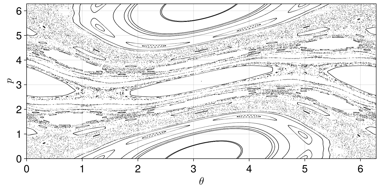

and finally, plot the fixed points

markers = [:diamond, :utriangle, :rect, :pentagon, :hexagon, :circle]

for i in 1:6
    FP = ALLFP[i]
    o = orders[i]
    scatter!(ax, columns(FP)...; marker=markers[i], color = Cycled(i),
        markersize = 30 - 2i, strokecolor = "grey", strokewidth = 1, label = "order $o"
    )
end
axislegend(ax)
fig

Okay, this output is great, and we can tell that it is correct because:

Fixed points of order $n$ are also fixed points of order $2n, 3n, 4n, ...$
Besides fixed points of previous orders, original fixed points of order $n$ come in (possible multiples of) $2n$-sized pairs (see e.g. order 5). This is a direct consequence of the Poincaré–Birkhoff theorem.

Davidchack & Lai

An extension of the previous algorithm was proposed by Davidchack & Lai (Davidchack and Lai, 1999). It works similarly, but it uses smarter seeding and an improved transformation rule.

The functions davidchacklai implements the algorithm:

ChaosTools.davidchacklai — Function

davidchacklai(ds::DeterministicIteratedMap, n::Int, ics, m::Int; kwargs...) -> fps

Find periodic orbits fps of orders 1 to n for the map ds using the algorithm propesed by Davidchack & Lai(Davidchack and Lai, 1999). ics is a collection of initial conditions (container of vectors) to be evolved. ics will be used to detect periodic orbits of orders 1 to m. These m periodic orbits will be used to detect periodic orbits of order m+1 to n. fps is a vector with n elements. i-th element is a periodic orbit of order i.

Keyword arguments

β = nothing: If it is nothing, then β(n) = 10*1.2^n. Otherwise can be a function that takes period n and return a number. It is a parameter mentioned in the paper(Davidchack and Lai, 1999).
maxiters = nothing: If it is nothing, then initial condition will be iterated max(100, 4*β(p)) times (where p is the order of the periodic orbit) before claiming it has not converged. If an integer, then it is the maximum amount of iterations an initial condition will be iterated before claiming it has not converged.
disttol = 1e-10: Distance tolerance. If norm(f^{n}(x)-x) < disttol where f^{n} is the n-th iterate of the dynamic rule f, then x is an n-periodic point.
abstol = 1e-8: A detected periodic point isn't stored if it is in abstol neighborhood of some previously detected point. Distance is measured by euclidian norm. If you are getting duplicate periodic points, increase this value.

Description

The algorithm is an extension of Schmelcher & Diakonos(Schmelcher and Diakonos, 1997) implemented in periodicorbits.

The algorithm can detect periodic orbits by turning fixed points of the original map ds to stable ones, through the transformation

\[\mathbf{x}_{n+1} = \mathbf{x}_{n} + [\beta |g(\mathbf{x}_{n})| C^{T} - J(\mathbf{x}_{n})]^{-1} g(\mathbf{x}_{n})\]

where

\[g(\mathbf{x}_{n}) = f^{n}(\mathbf{x}_{n}) - \mathbf{x}_{n}\]

and

\[J(\mathbf{x}_{n}) = \frac{\partial g(\mathbf{x}_{n})}{\partial \mathbf{x}_{n}}\]

The main difference between Schmelcher & Diakonos(Schmelcher and Diakonos, 1997) and Davidchack & Lai(Davidchack and Lai, 1999) is that the latter uses periodic points of previous period as seeds to detect periodic points of the next period. Additionally, periodicorbits only detects periodic points of a given order, while davidchacklai detects periodic points of all orders up to n.

Important note

For low periods n circa less than 6, you should select m = n otherwise the algorithm won't detect periodic orbits correctly. For higher periods, you can select m as 6. We recommend experimenting with m as it may depend on the specific problem. Increase m in case the orbits are not being detected correctly.

Initial conditions ics can be selected as a uniform grid of points in the state space or subset of a chaotic trajectory.

source

Logistic Map example

The idea of periodic orbits can be illustrated easily on 1D maps. Finding all periodic orbits of period $n$ is equivalent to finding all points $x$ such that $f^{n}(x)=x$, where $f^{n}$ is $n$-th composition of $f$. Hence, solving $f^{n}(x)-x=0$ yields such points. However, this is often impossible analytically. Let's see how davidchacklai deals with it:

First let's start with finding first $9$ periodic orbits of the logistic map for parameter $3.72$.

using ChaosTools
using CairoMakie

logistic_rule(x, p, n) = @inbounds SVector(p[1]*x[1]*(1 - x[1]))
ds = DeterministicIteratedMap(logistic_rule, SVector(0.4), [3.72])
seeds = [SVector(i) for i in LinRange(0.0, 1.0, 10)]
output = davidchacklai(ds, 9, seeds, 6; abstol=1e-6, disttol=1e-12)

9-element Vector{Vector{SVector{1, Float64}}}:
 [[0.7311827956985908], [0.0]]
 [[0.38662970705800187], [0.7311827956989247], [0.0], [0.8821874972430735]]
 [[0.7311827956989247], [0.0]]
 [[0.3177034818396079], [0.5808155232915662], [0.0], [0.38662970705800176], [0.806376883615744], [0.9057041264458106], [0.8821874972430734], [0.73118279569892]]
 [[0.0], [0.7311827956989269]]
 [[0.9157520118590331], [0.6299077421471525], [0.286998984442819], [0.9109040211331463], [0.8672212001324516], [0.3866297070580018], [0.7840245795497282], [0.5618878367611084], [0.30190733374979245], [0.8821874972430734], [0.8145709500114354], [0.6761513965685626], [0.7311827956989247], [0.0], [0.7612257106223875], [0.4283527554446087]]
 [[0.7767552610676709], [0.8517090105640062], [0.6674116032936027], [0.8257408809075153], [0.46983887142368663], [0.7656845473197781], [0.9253694005081607], [0.645072274753479], [0.25295568534359186], [0.2569064479741398], [0.7029650765369176], [0.7311827956989247], [0.7101685528640355], [0.0], [0.9266159395216157], [0.5352815080408169]]
 [[0.580815523291563], [0.2752211565830479], [0.37176048427534275], [0.8873814476036359], [0.27922483081767735], [0.9195423913299305], [0.868823210976944], [0.6356815832652796], [0.9057041264458124], [0.7120608293260391]  …  [0.9182577693338777], [0.6732538405098987], [0.8821874972430507], [0.7946496422194083], [0.7311827956989247], [0.38662970705800187], [0.0], [0.31770348183960895], [0.8063768836157453], [0.3092527725503487]]
 [[0.8351397865800463], [0.2439348271350769], [0.7244574163099475], [0.9233919394296619], [0.5925398344373891], [0.5969310175617724], [0.64079266064647], [0.5439224240213731], [0.7642367356877261], [0.929448625260208]  …  [0.7015891525631268], [0.8011894723749792], [0.8562600273540872], [0.45785310962395387], [0.7311827956989247], [0.742582189940082], [0.0], [0.3403126261379589], [0.8950482855441152], [0.9228234528852824]]

Now to check the results, let's plot the periodic orbits of period $6$, $7$, $8$ and $9$.

function ydata(ds, order, xdata)
    ydata = typeof(current_state(ds)[1])[]
    for x in xdata
        reinit!(ds, x)
        step!(ds, order)
        push!(ydata, current_state(ds)[1])
    end
    return ydata
end

fig = Figure()
x = LinRange(0.0, 1.0, 1000)
for (order, position)  in zip([6,7,8,9], [(1,1), (1,2), (2,1), (2,2)])
    fpsx = output[order]
    y = ydata(ds, order, [SVector(x0) for x0 in x])
    fpsy = ydata(ds, order, fpsx)
    axis = Axis(fig[position...])
    axis.title = "Order $order"
    lines!(axis, x, x, color=:black, linewidth=0.5)
    lines!(axis, x, y, color = :blue, linewidth=0.7)
    scatter!(axis, [i[1] for i in fpsx], fpsy, color = :red, markersize=5)
end
fig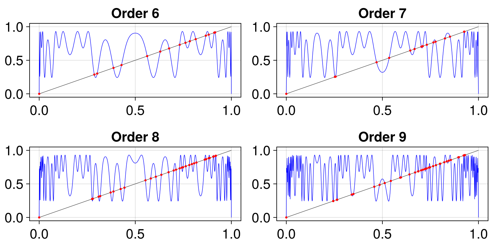

Points $x$ which fulfill $f^{n}(x)=x$ can be interpreted as an intersection of the function $f^{n}(x)$ and the identity $x$. Our result is correct because all the points of the intersection between the identity and the logistic map were found.

Henon Map example

Let's try to use davidchacklai in higher dimension. We will try to detect all periodic points of Henon map of period 1 to 14.

using ChaosTools, CairoMakie

function henon(u0=zeros(2); a = 1.4, b = 0.3)
    return DeterministicIteratedMap(henon_rule, u0, [a,b])
end
henon_rule(x, p, n) = SVector{2}(1.0 - p[1]*x[1]^2 + x[2], p[2]*x[1])

ds = henon()
xs = LinRange(-3.0, 3.0, 10)
ys = LinRange(-10.0, 10.0, 10)
seeds = [SVector{2}(x,y) for x in xs for y in ys]
n = 14
m = 6
output = davidchacklai(ds, n, seeds, m; abstol=1e-7, disttol=1e-10)

fig = Figure()
ax = Axis(fig[1,1])
for result in output
    scatter!(ax, [x[1] for x in result], [x[2] for x in result], markersize=8, color=:blue)
end
fig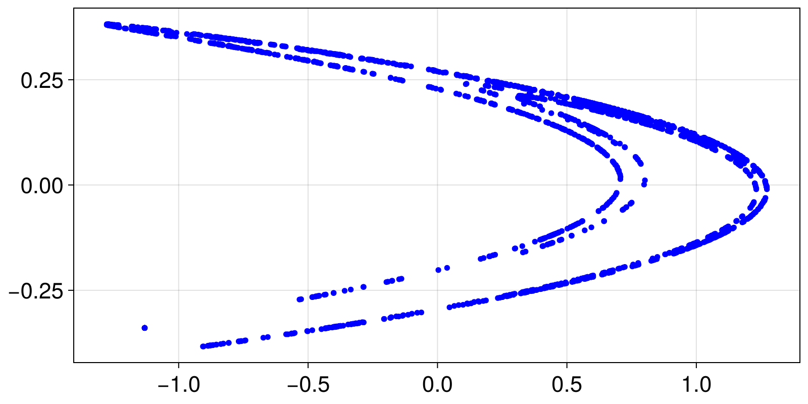

The theory of periodic orbits states that UPOs form sort of a skeleton of the chaotic attractor. Our results supports this claim since it closely resembles the Henon attractor.

Note that in this case parameter m has to be set to at least 6. Otherwise, the algorithm fails to detect orbits of higher periods correctly.

To check if the detected points are indeed periodic, we can do the following test:

    orbit14 = output[end]
    c = 0
    for x in orbit14
        set_state!(ds, x)
        step!(ds, 14)
        xn = current_state(ds)
        if ChaosTools.norm(xn - x) > 1e-10
            c += 1
        end
    end
    "$c non-periodic points found in the 14th order orbit."

"0 non-periodic points found in the 14th order orbit."

The same test can be applied to orbits of lower periods.

Estimating the Period

The function estimate_period offers ways for estimating the period (either exact for periodic timeseries, or approximate for near-periodic ones) of a given timeseries. We offer five methods to estimate periods, some of which work on evenly sampled data only, and others which accept any data. The figure below summarizes this:

ChaosTools.estimate_period — Function

estimate_period(v::Vector, method, t=0:length(v)-1; kwargs...)

Estimate the period of the signal v, with accompanying time vector t, using the given method.

If t is an AbstractArray, then it is iterated through to ensure that it's evenly sampled (if necessary for the algorithm). To avoid this, you can pass any AbstractRange, like a UnitRange or a LinRange, which are defined to be evenly sampled.

Methods requiring evenly sampled data

These methods are faster, but some are error-prone.

:periodogram or :pg: Use the fast Fourier transform to compute a periodogram (power-spectrum) of the given data. Data must be evenly sampled.
:multitaper or mt: The multitaper method reduces estimation bias by using multiple independent estimates from the same sample. Data tapers are then windowed and the power spectra are obtained. Available keywords follow: nw is the time-bandwidth product, and ntapers is the number of tapers. If window is not specified, the signal is tapered with ntapers discrete prolate spheroidal sequences with time-bandwidth product nw. Each sequence is equally weighted; adaptive multitaper is not (yet) supported. If window is specified, each column is applied as a taper. The sum of periodograms is normalized by the total sum of squares of window.
:autocorrelation or :ac: Use the autocorrelation function (AC). The value where the AC first comes back close to 1 is the period of the signal. The keyword L = length(v)÷10 denotes the length of the AC (thus, given the default setting, this method will fail if there less than 10 periods in the signal). The keyword ϵ = 0.2 (\epsilon) means that 1-ϵ counts as "1" for the AC.
:yin: The YIN algorithm. An autocorrelation-based method to estimate the fundamental period of the signal. See the original paper ^{[CheveigneYIN2002]} or the implementation yin. Sampling rate is taken as sr = 1/mean(diff(t)) if not given.

speech and music. The Journal of the Acoustical Society of America, 111(4), 1917-1930.

Methods not requiring evenly sampled data

These methods tend to be slow, but versatile and low-error.

:lombscargle or :ls: Use the Lomb-Scargle algorithm to compute a periodogram. The advantage of the Lomb-Scargle method is that it does not require an equally sampled dataset and performs well on undersampled datasets. Constraints have been set on the period, since Lomb-Scargle tends to have false peaks at very low frequencies. That being said, it's a very flexible method. It is extremely customizable, and the keyword arguments that can be passed to it are given in the documentation.
:zerocrossing or :zc: Find the zero crossings of the data, and use the average difference between zero crossings as the period. This is a naïve implementation, with only linear interpolation; however, it's useful as a sanity check. The keyword line controls where the "crossing point" is. It defaults to mean(v).

For more information on the periodogram methods, see the documentation of DSP.jl and LombScargle.jl.

source

ChaosTools.yin — Function

yin(sig::Vector, sr::Int; kwargs...) -> F0s, frame_times

Estimate the fundamental frequency (F0) of the signal sig using the YIN algorithm ^[1]. The signal sig is a vector of points uniformly sampled at a rate sr.

Keyword arguments

w_len: size of the analysis window [samples == number of points]
f_step: size of the lag between two consecutive frames [samples == number of points]
f0_min: Minimum fundamental frequency that can be detected [linear frequency]
f0_max: Maximum fundamental frequency that can be detected [linear frequency]
harmonic_threshold: Threshold of detection. The algorithm returns the first minimum of the CMNDF function below this threshold.
diffference_function: The difference function to be used (by default ChaosTools.difference_function_original).

Description

The YIN algorithm ^{[CheveigneYIN2002]} estimates the signal's fundamental frequency F0 by basically looking for the period τ0 which minimizes the signal's autocorrelation. This autocorrelation is calculated for signal segments (frames), composed of two windows of length w_len. Each window is separated by a distance τ, and the idea is that the distance which minimizes the pairwise difference between each window is considered to be the fundamental period τ0 of that frame.

More precisely, the algorithm first computes the cumulative mean normalized difference function (MNDF) between two windows of a frame for several candidate periods τ ranging from τ_min=sr/f0_max to τ_max=sr/f0_min. The MNDF is defined as

\[d_t^\prime(\tau) = \begin{cases} 1 & \text{if} ~ \tau=0 \\ d_t(\tau)/\left[{(\frac 1 \tau) \sum_{j=1}^{\tau} d_{t}(j)}\right] & \text{otherwise} \end{cases}\]

where d_t is the difference function:

\[d_t(\tau) = \sum_{j=1}^W (x_j - x_{j+\tau})^2\]

It then refines the local minima of the MNDF using parabolic (quadratic) interpolation. This is done by taking each minima, along with their first neighbor points, and finding the minimum of the corresponding interpolated parabola. The MNDF minima are substituted by the interpolation minima. Finally, the algorithm chooses the minimum with the smallest period and with a corresponding MNDF below the harmonic threshold. If this doesn't exist, it chooses the period corresponding to the global minimum. It repeats this for frames starting at the first signal point, and separated by a distance f_step (frames can overlap), and returns the vector of frequencies F0=sr/τ0 for each frame, along with the start times of each frame.

As a note, the physical unit of the frequency is 1/[time], where [time] is decided by the sampling rate sr. If, for instance, the sampling rate is over seconds, then the frequency is in Hertz.

speech and music. The Journal of the Acoustical Society of America, 111(4), 1917-1930.

source

Example

Here we will use a modified FitzHugh-Nagumo system that results in periodic behavior, and then try to estimate its period. First, let's see the trajectory:

using ChaosTools, CairoMakie

function FHN(u, p, t)
    e, b, g = p
    v, w = u
    dv = min(max(-2 - v, v), 2 - v) - w
    dw = e*(v - g*w + b)
    return SVector(dv, dw)
end

g, e, b  = 0.8, 0.04, 0.0
p0 = [e, b, g]

fhn = CoupledODEs(FHN, SVector(-2, -0.6667), p0)
T, Δt = 1000.0, 0.1
X, t = trajectory(fhn, T; Δt)
v = X[:, 1]

lines(t, v)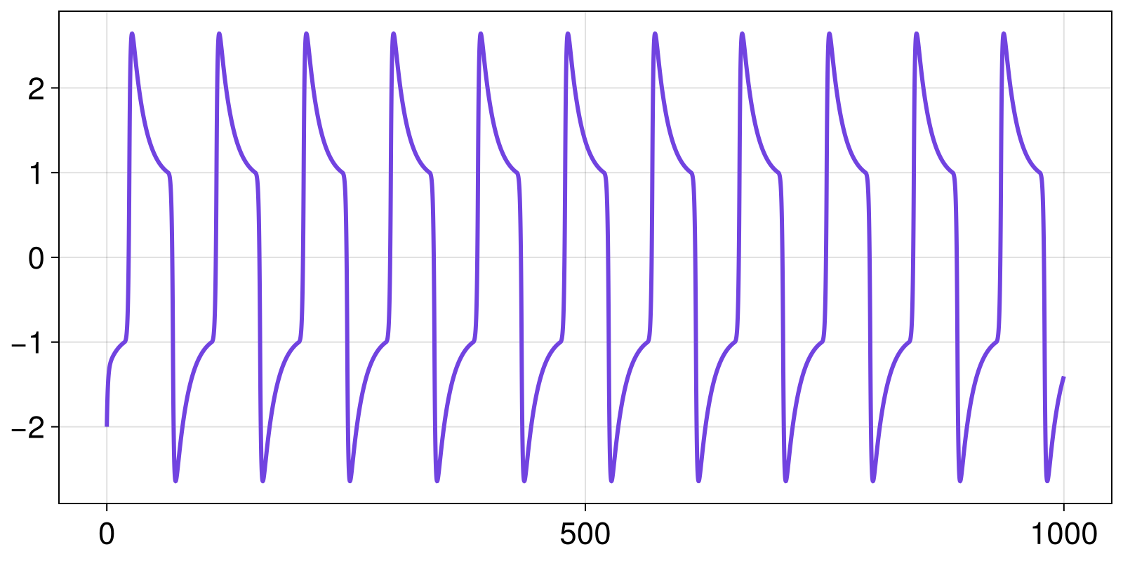

Examining the figure, one can see that the period of the system is around 91 time units. To estimate it numerically let's use some of the methods:

estimate_period(v, :autocorrelation, t)

91.0

estimate_period(v, :periodogram, t)

91.62720091627202

estimate_period(v, :zerocrossing, t)

91.08000000000001

estimate_period(v, :yin, t; f0_min=0.01)

91.07387792483064

Schmelcher1997P. Schmelcher & F. K. Diakonos, Phys. Rev. Lett. 78, pp 4733 (1997)
Pingel2000D. Pingel et al., Phys. Rev. E 62, pp 2119 (2000)
Diakonos1998F. K. Diakonos et al., Phys. Rev. Lett. 81, pp 4349 (1998)
CheveigneYIN2002De Cheveigné, A., & Kawahara, H. (2002). YIN, a fundamental frequency estimator for
CheveigneYIN2002De Cheveigné, A., & Kawahara, H. (2002). YIN, a fundamental frequency estimator for