Daisyworld

Study this example to learn about

• Simple agent properties with complex model interactions
• Diffusion of a quantity in a grid space
• Including a "surface property" in the model
• counting time in the model and having time-dependent dynamics
• performing interactive scientific research

Overview of Daisyworld

This model explores the Gaia hypothesis, which considers the Earth as a single, self-regulating system including both living and non-living parts.

Daisyworld is filled with black and white daisies. Their albedo's differ, with black daisies absorbing light and heat, warming the area around them; white daisies doing the opposite. Daisies can only reproduce within a certain temperature range, meaning too much (or too little) heat coming from the sun and/or surrounds will ultimately halt daisy propagation.

When the climate is too cold it is necessary for the black daisies to propagate in order to raise the temperature, and vice versa – when the climate is too warm, it is necessary for more white daisies to be produced in order to cool the temperature. The interplay of the living and non living aspects of this world manages to find an equilibrium over a wide range of parameter settings, although with enough external forcing, the daisies will not be able to regulate the temperature of the planet and eventually go extinct.

Defining the daisy type

Daisy has three values (other than the required id and pos for an agent that lives on a GridSpaceSingle. Each daisy has an age, confined later by a maximum age set by the user, a breed (either :black or :white) and an associated albedo value, again set by the user.

using Agents
using Random
import StatsBase

@agent struct Daisy(GridAgent{2})
    breed::Symbol
    age::Int
    albedo::Float64 # 0-1 fraction
end

World heating

Notice that the surface is not an agent but rather a standard Julia array. This is something we typically instruct Agents.jl users to do: not make surface properties agents (even though this is done in other ABM frameworks) because it is simply much more performant to use standard arrays. Hence, here the surface temperature will be a matrix with same size as the grid.

The surface temperature of the world is heated by its sun, but daisies growing upon it absorb or reflect the starlight, altering the local temperature.

function update_surface_temperature!(pos, model)
    absorbed_luminosity = if isempty(pos, model) # no daisy
        # Set luminosity via surface albedo
        (1 - model.surface_albedo) * model.solar_luminosity
    else
        daisy = model[id_in_position(pos, model)]
        # Set luminosity via daisy albedo
        (1 - daisy.albedo) * model.solar_luminosity
    end
    # We expect local heating to be 80 ᵒC for an absorbed luminosity of 1,
    # approximately 30 for 0.5 and approximately -273 for 0.01.
    local_heating = absorbed_luminosity > 0 ? 72 * log(absorbed_luminosity) + 80 : 80
    # Surface temperature is the average of the current temperature and local heating.
    model.temperature[pos...] = (model.temperature[pos...] + local_heating) / 2
end

update_surface_temperature! (generic function with 1 method)

In addition, temperature diffuses over time

function diffuse_temperature!(pos, model)
    ratio = model.ratio # diffusion ratio
    npos = nearby_positions(pos, model)
    model.temperature[pos...] =
        (1 - ratio) * model.temperature[pos...] +
        # Each neighbor is giving up 1/8 of the diffused
        # amount to each of *its* neighbors
        sum(model.temperature[p...] for p in npos) * 0.125 * ratio
end

diffuse_temperature! (generic function with 1 method)

Daisy dynamics

The final piece of the puzzle is the life-cycle of each daisy. This method defines an optimal temperature for growth. If the temperature gets too hot or too cold, daisies will not wish to propagate. So long as the temperature is favorable, daisies compete for land and attempt to spawn a new plant of their breed in locations close to them.

function propagate!(pos, model)
    isempty(pos, model) && return
    daisy = model[id_in_position(pos, model)]
    temperature = model.temperature[pos...]
    seed_threshold = (0.1457 * temperature - 0.0032 * temperature^2) - 0.6443
    if rand(abmrng(model)) < seed_threshold
        empty_near_pos = random_nearby_position(pos, model, 1, npos -> isempty(npos, model))
        if !isnothing(empty_near_pos)
            add_agent!(empty_near_pos, model, daisy.breed, 0, daisy.albedo)
        end
    end
end

propagate! (generic function with 1 method)

And if the daisies cross an age threshold, they die out. Death is controlled by the agent_step! function

function daisy_step!(agent::Daisy, model)
    agent.age += 1
    agent.age ≥ model.max_age && remove_agent!(agent, model)
end

daisy_step! (generic function with 1 method)

The model step function advances Daisyworld's dynamics:

function daisyworld_step!(model)
    for p in positions(model)
        update_surface_temperature!(p, model)
        diffuse_temperature!(p, model)
        propagate!(p, model)
    end
    solar_activity!(model)
end

daisyworld_step! (generic function with 1 method)

Notice that solar_activity! changes the incoming solar radiation over time, if the given "scenario" (a model parameter) is :ramp.

function solar_activity!(model)
    if model.scenario == :ramp
        if 200 < abmtime(model) ≤ 400
            model.solar_luminosity += model.solar_change
        end
        if 500 < abmtime(model) ≤ 750
            model.solar_luminosity -= model.solar_change / 2
        end
    elseif model.scenario == :change
        model.solar_luminosity += model.solar_change
    end
end

solar_activity! (generic function with 1 method)

Initialising Daisyworld

Here, we construct a function to initialize a Daisyworld. We use fill_space! to fill the space with Land instances. Then, we need to know how many daisies of each type to seed the planet with and what their albedo's are. We also want a value for surface albedo, as well as solar intensity (and we also choose between constant or time-dependent intensity with scenario).

function daisyworld(;
    griddims = (30, 30),
    max_age = 25,
    init_white = 0.2, # % cover of the world surface of white breed
    init_black = 0.2, # % cover of the world surface of black breed
    albedo_white = 0.75,
    albedo_black = 0.25,
    surface_albedo = 0.4,
    solar_change = 0.005,
    solar_luminosity = 1.0, # initial luminosity
    scenario = :default,
    seed = 165,
)
    rng = MersenneTwister(seed)
    space = GridSpaceSingle(griddims)
    # Here the model properties is a `NamedTuple`, which avoid type instabilities.
    # However, `NamedTuple`s can't be mutated, and hence we would not be able
    # to use this in an interactive application. The correct way is to
    # Create a custom `struct`, but here we'll be lazy and make a abstract
    # typed dictionary
    properties = (;max_age, surface_albedo, solar_luminosity, solar_change, scenario,
        ratio = 0.5, temperature = zeros(griddims)
    )
    properties = Dict(k=>v for (k,v) in pairs(properties))

    model = StandardABM(Daisy, space; properties, rng, agent_step! = daisy_step!, model_step! = daisyworld_step!)

    # Populate with daisies: each position has only one daisy (black or white)
    grid = collect(positions(model))
    num_positions = prod(griddims)
    white_positions =
        StatsBase.sample(grid, Int(init_white * num_positions); replace = false)
    for wp in white_positions
        add_agent!(wp, Daisy, model, :white, rand(abmrng(model), 0:max_age), albedo_white)
    end
    allowed = setdiff(grid, white_positions)
    black_positions =
        StatsBase.sample(allowed, Int(init_black * num_positions); replace = false)
    for bp in black_positions
        add_agent!(bp, Daisy, model, :black, rand(abmrng(model), 0:max_age), albedo_black)
    end

    # Adjust temperature to initial daisy distribution
    for p in positions(model)
        update_surface_temperature!(p, model)
    end

    return model
end

daisyworld (generic function with 1 method)

Visualizing & animating

Lets run the model with constant solar isolation and visualize the result

using CairoMakie
model = daisyworld()

StandardABM with 360 agents of type Daisy
 agents container: Dict
 space: GridSpaceSingle with size (30, 30), metric=chebyshev, periodic=true
 scheduler: fastest
 properties: temperature, solar_luminosity, max_age, surface_albedo, ratio, solar_change, scenario

To visualize we need to define the necessary functions for abmplot. We will also utilize its ability to plot an underlying heatmap, which will be the model surface temperature, while daisies will be plotted in black and white as per their breed. Notice that we will explicitly provide a colorrange to the heatmap keywords, otherwise the colormap will be continuously and automatically updated to match the underlying temperature values while we are animating the time evolution.

daisycolor(a::Daisy) = a.breed

plotkwargs = (
    agent_color=daisycolor, agent_size = 20, agent_marker = '✿',
    heatarray = :temperature,
    heatkwargs = (colorrange = (-20, 60),),
)
fig, _ = abmplot(model; plotkwargs...)
fig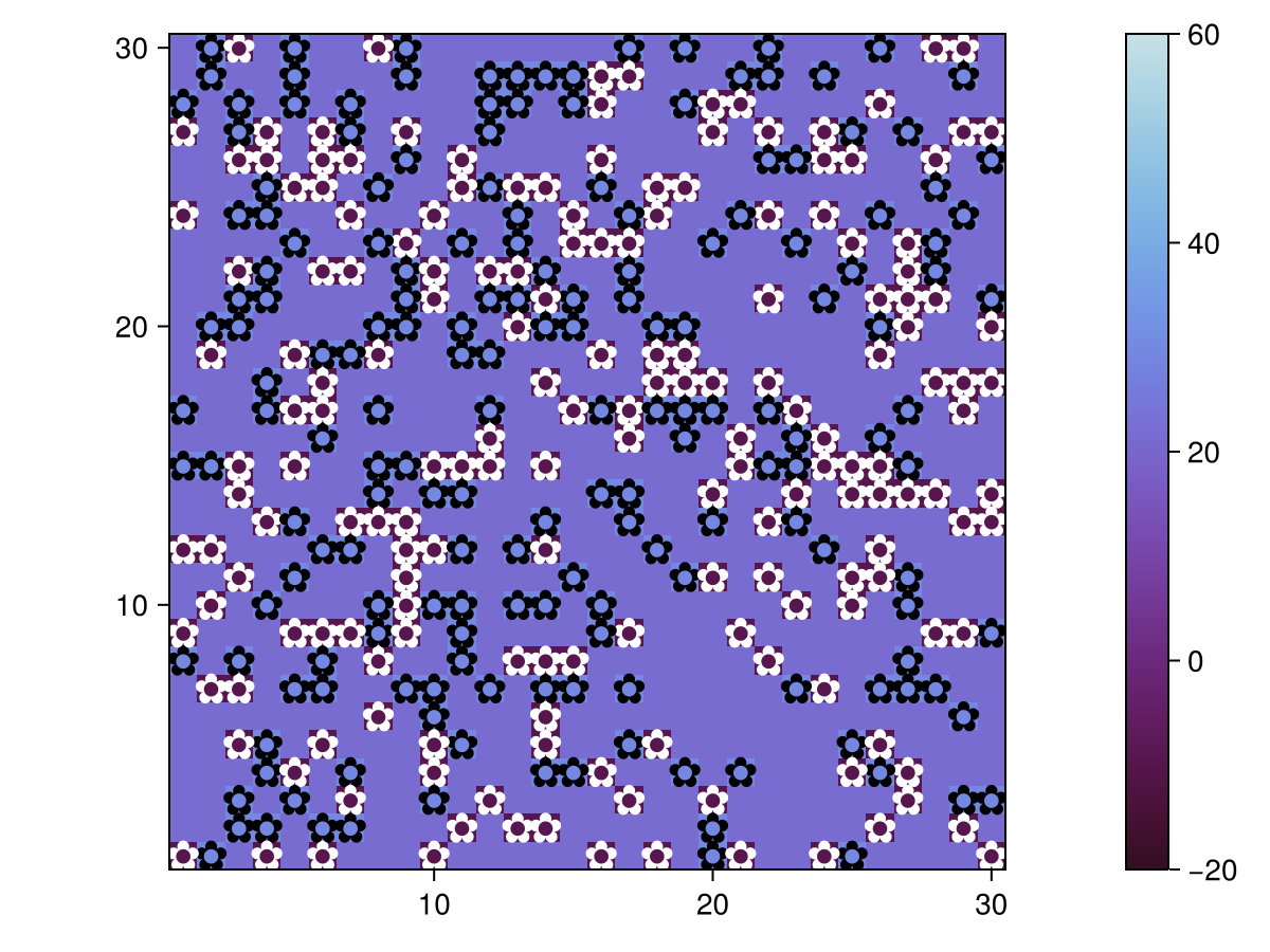

And after a couple of steps

step!(model, 5)
fig, _ = abmplot(model; heatarray = model.temperature, plotkwargs...)
fig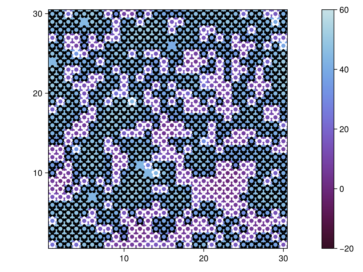

Let's do some animation now

model = daisyworld()
abmvideo(
    "daisyworld.mp4",
    model;
    title = "Daisy World",
    frames = 60,
    plotkwargs...,
)

Running this animation for longer hints that this world achieves quasi-equilibrium for some input parameters, where one breed does not totally dominate the other. Of course we can check this easily through data collection. Notice that here we have to define a function breed that returns the daisy's breed field. We cannot use just :breed to automatically find it, because in this mixed agent model, the Land doesn't have any breed.

black(a) = a.breed == :black
white(a) = a.breed == :white
adata = [(black, count), (white, count)]

model = daisyworld(; solar_luminosity = 1.0)

agent_df, model_df = run!(model, 1000; adata)
figure = Figure(size = (600, 400));
ax = figure[1, 1] = Axis(figure, xlabel = "tick", ylabel = "daisy count")
blackl = lines!(ax, agent_df[!, :time], agent_df[!, :count_black], color = :black)
whitel = lines!(ax, agent_df[!, :time], agent_df[!, :count_white], color = :orange)
Legend(figure[1, 2], [blackl, whitel], ["black", "white"], labelsize = 12)
figure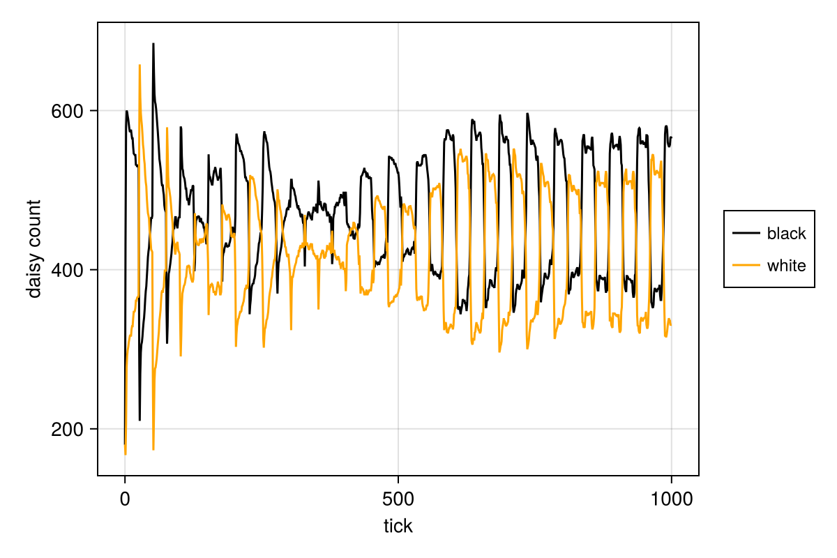

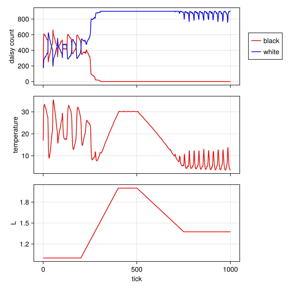
Time dependent dynamics

To use the time-dependent dynamics we simply use the keyword scenario = :ramp during model creation. However, we also want to see how the planet surface temperature changes and would be nice to plot solar luminosity as well. Thus, we define in addition

temperature(model) = StatsBase.mean(model.temperature)
mdata = [temperature, :solar_luminosity]

2-element Vector{Any}:
 temperature (generic function with 1 method)
 :solar_luminosity

And we run (and plot) everything

model = daisyworld(solar_luminosity = 1.0, scenario = :ramp)
agent_df, model_df = run!(model, 1000; adata = adata, mdata = mdata)

figure = CairoMakie.Figure(size = (600, 600));
ax1 = figure[1, 1] = Axis(figure, ylabel = "daisy count")
blackl = lines!(ax1, agent_df[!, :time], agent_df[!, :count_black], color = :red)
whitel = lines!(ax1, agent_df[!, :time], agent_df[!, :count_white], color = :blue)
figure[1, 2] = Legend(figure, [blackl, whitel], ["black", "white"])

ax2 = figure[2, 1] = Axis(figure, ylabel = "temperature")
ax3 = figure[3, 1] = Axis(figure, xlabel = "tick", ylabel = "L")
lines!(ax2, model_df[!, :time], model_df[!, :temperature], color = :red)
lines!(ax3, model_df[!, :time], model_df[!, :solar_luminosity], color = :red)
for ax in (ax1, ax2); ax.xticklabelsvisible = false; end
figure