Continuous space social distancing
This is a model similar to our SIR model for the spread of COVID-19. But instead of having different cities, we let agents move in one continuous space and transfer the disease if they come into contact with one another. This model is partly inspired by this article, and can complement the SIR graph model. The graph model can model virus transfer between cities, whilst this model can be used to study what happens within a city.
The example here serves additionally as an introduction to using continuous space, modelling billiard-like collisions in that space, and animating the agent motion in the space. Notice that a detailed description of the basics of the model regarding disease spreading exists in the SIR example, and is not repeated here.
It is also available from the Models module as Models.social_distancing.
Moving agents in continuous space
Let us first create a simple model where balls move around in a continuous space. We need to create agents that comply with ContinuousSpace, i.e. they have a pos and vel fields, both of which are tuples of float numbers.
using Agents, Random

@agent struct SocialAgent(ContinuousAgent{2, Float64})
    mass::Float64
end
The mass field will come in handy later on, when we implement social isolation (i.e. that some agents don't move and can't be moved).
Let's also initialize a trivial model with continuous space
function ball_model(; speed = 0.002)
    space2d = ContinuousSpace((1, 1); spacing = 0.02)
    model = StandardABM(SocialAgent, space2d; agent_step!, properties = Dict(:dt => 1.0),
                        rng = MersenneTwister(42))
    # And add some agents to the model
    for ind in 1:500
        pos = Tuple(rand(abmrng(model), 2))
        vel = sincos(2π * rand(abmrng(model))) .* speed
        add_agent!(pos, model, vel, 1.0)
    end
    return model
end
ball_model (generic function with 1 method)We took advantage of the functionality of add_agent! that creates the agents automatically. For now all agents have the same absolute speed, and mass.
The agent step function for now is trivial. It is just move_agent! in continuous space
agent_step!(agent, model) = move_agent!(agent, model, model.dt)agent_step! (generic function with 1 method)dt is our time resolution, but we will talk about this more later!
Billiard-like interaction
We will model the agents as balls that collide with each other. To this end, we will use two functions from the continuous space API:
We want all agents to interact in one go, and we want to avoid double interactions (as instructed by interacting_pairs), so we define a model step.
function model_step!(model)
    for (a1, a2) in interacting_pairs(model, 0.012, :nearest)
        elastic_collision!(a1, a2, :mass)
    end
end

model = ball_model()
StandardABM with 500 agents of type SocialAgent
agents container: Dict
space: periodic continuous space with [1.0, 1.0] extent and spacing=0.02
scheduler: fastest
properties: dtAnd then make an animation
using CairoMakie

abmvideo(
    "socialdist2.mp4",
    model;
    title = "Billiard-like",
    frames = 50,
    spf = 2,
    framerate = 25,
)
┌ Warning: keyword `spf` is deprecated in favor of `dt`.
└ @ AgentsVisualizations ~/.julia/packages/Agents/eKASH/ext/AgentsVisualizations/src/convenience.jl:102Alright, this works great so far!
Please understand that Agents.jl does not accurately simulate billiard systems. This is the job of Julia packages HardSphereDynamics.jl or DynamicalBilliards.jl. In Agents.jl we only provide an approximating function elastic_collision!. The accuracy of this simulation increases as the time resolution dt decreases, but even in the limit dt → 0 we still don't reach the accuracy of proper billiard packages.
Also notice that the plotted size of the circles representing agents is not deduced from the interaction_radius (as it should). We only eye-balled it to look similar enough.
Immovable agents
For the following social distancing example, it will become crucial that some agents don't move, and can't be moved (i.e. they stay "isolated"). This is very easy to do with the elastic_collision! function, we only have to make some agents have infinite mass
model2 = ball_model()

for id in 1:400
    agent = model2[id]
    agent.mass = Inf
    agent.vel = (0.0, 0.0)
end
let's animate this again
abmvideo(
    "socialdist3.mp4",
    model2;
    title = "Billiard-like with stationary agents",
    frames = 50,
    spf = 2,
    framerate = 25,
)
┌ Warning: keyword `spf` is deprecated in favor of `dt`.
└ @ AgentsVisualizations ~/.julia/packages/Agents/eKASH/ext/AgentsVisualizations/src/convenience.jl:102Adding Virus spread (SIR)
We now add more functionality to these agents, according to the SIR model (see previous example). They can be infected with a disease and transfer the disease to other agents around them.
@agent struct PoorSoul(ContinuousAgent{2, Float64})
    mass::Float64
    days_infected::Int  # number of days since is infected
    status::Symbol  # :S, :I or :R
    β::Float64
end
Here β is the transmission probability, which we choose to make an agent parameter instead of a model parameter. It reflects the level of hygiene of an individual. In a realistic scenario, the actual virus transmission would depend on the β value of both agents, but we don't do that here for simplicity.
We also significantly modify the model creation, to have SIR-related parameters. Each step in the model corresponds to one hour.
const steps_per_day = 24

using DrWatson: @dict
function sir_initiation(;
    infection_period = 30 * steps_per_day,
    detection_time = 14 * steps_per_day,
    reinfection_probability = 0.05,
    isolated = 0.0, # in percentage
    interaction_radius = 0.012,
    dt = 1.0,
    speed = 0.002,
    death_rate = 0.044, # from website of WHO
    N = 1000,
    initial_infected = 5,
    seed = 42,
    βmin = 0.4,
    βmax = 0.8,
)

    properties = (;
        infection_period,
        reinfection_probability,
        detection_time,
        death_rate,
        interaction_radius,
        dt,
    )
    space = ContinuousSpace((1,1); spacing = 0.02)
    model = StandardABM(PoorSoul, space, agent_step! = sir_agent_step!,
                        model_step! = sir_model_step!, properties = properties,
                        rng = MersenneTwister(seed))

    # Add initial individuals
    for ind in 1:N
        pos = Tuple(rand(abmrng(model), 2))
        status = ind ≤ N - initial_infected ? :S : :I
        isisolated = ind ≤ isolated * N
        mass = isisolated ? Inf : 1.0
        vel = isisolated ? (0.0, 0.0) : sincos(2π * rand(abmrng(model))) .* speed

        # very high transmission probability
        # we are modelling close encounters after all
        β = (βmax - βmin) * rand(abmrng(model)) + βmin
        add_agent!(pos, model, vel, mass, 0, status, β)
    end

    return model
end
sir_initiation (generic function with 1 method)We have increased the size of the model 10-fold (for more realistic further analysis)
To actually spread the virus, we modify the model_step! function, so that individuals have a probability to transmit the disease as they interact.
function transmit!(a1, a2, rp)
    # for transmission, only 1 can have the disease (otherwise nothing happens)
    count(a.status == :I for a in (a1, a2)) ≠ 1 && return
    infected, healthy = a1.status == :I ? (a1, a2) : (a2, a1)

    rand(abmrng(model)) > infected.β && return

    if healthy.status == :R
        rand(abmrng(model)) > rp && return
    end
    healthy.status = :I
end

function sir_model_step!(model)
    r = model.interaction_radius
    for (a1, a2) in interacting_pairs(model, r, :nearest)
        transmit!(a1, a2, model.reinfection_probability)
        elastic_collision!(a1, a2, :mass)
    end
end
sir_model_step! (generic function with 1 method)Notice that it is not necessary that the transmission interaction radius is the same as the billiard-ball dynamics. We only have them the same here for convenience, but in a real model they will probably differ.
We also modify the agent_step! function, so that we keep track of how long the agent has been infected, and whether they have to die or not.
function sir_agent_step!(agent, model)
    move_agent!(agent, model, model.dt)
    update!(agent)
    recover_or_die!(agent, model)
end

update!(agent) = agent.status == :I && (agent.days_infected += 1)

function recover_or_die!(agent, model)
    if agent.days_infected ≥ model.infection_period
        if rand(abmrng(model)) ≤ model.death_rate
            remove_agent!(agent, model)
        else
            agent.status = :R
            agent.days_infected = 0
        end
    end
end
recover_or_die! (generic function with 1 method)Notice the constant steps_per_day, which approximates how many model steps correspond to one day (since the parameters we used in the previous graph SIR example were given in days).
To visualize this model, we will use black color for the susceptible, red for the infected infected and green for the recovered, leveraging InteractiveDynamics.abmplot.
sir_model = sir_initiation()

sir_colors(a) = a.status == :S ? "#2b2b33" : a.status == :I ? "#bf2642" : "#338c54"

fig, ax, abmp = abmplot(sir_model; ac = sir_colors)
fig # display figure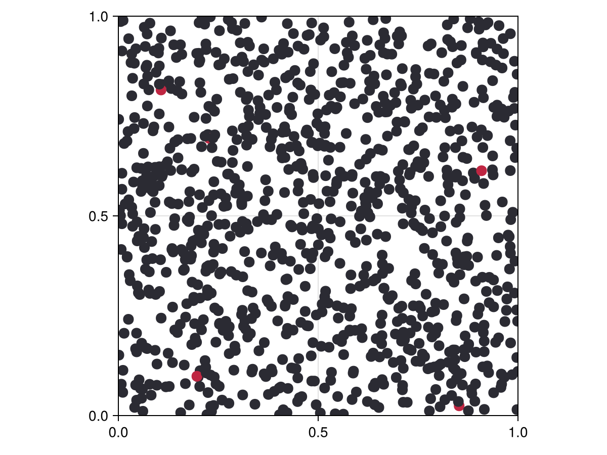
Alright, now we can animate this process for default parameters
sir_model = sir_initiation()

abmvideo(
    "socialdist4.mp4",
    sir_model;
    title = "SIR model",
    frames = 50,
    ac = sir_colors,
    as = 10,
    spf = 1,
    framerate = 20,
)
┌ Warning: keyword `spf` is deprecated in favor of `dt`.
└ @ AgentsVisualizations ~/.julia/packages/Agents/eKASH/ext/AgentsVisualizations/src/convenience.jl:102
┌ Warning: Keywords `as, am, ac` has been deprecated in favor of
│ `agent_size, agent_marker, agent_color`
└ @ AgentsVisualizations ~/.julia/packages/Agents/eKASH/ext/AgentsVisualizations/src/abmplot.jl:70Exponential spread
We can all agree that these animations look interesting, but let's do some actual analysis of this model. The quantity we wish to look at is the number of infected over time, so let's calculate this, similarly with the graph SIR model.
infected(x) = count(i == :I for i in x)
recovered(x) = count(i == :R for i in x)
adata = [(:status, infected), (:status, recovered)]
2-element Vector{Tuple{Symbol, Function}}:
(:status, Main.infected)
(:status, Main.recovered)Let's do the following runs, with different parameters probabilities
r1, r2 = 0.04, 0.33
β1, β2 = 0.5, 0.1
sir_model1 = sir_initiation(reinfection_probability = r1, βmin = β1)
sir_model2 = sir_initiation(reinfection_probability = r2, βmin = β1)
sir_model3 = sir_initiation(reinfection_probability = r1, βmin = β2)

data1, _ = run!(sir_model1, 2000; adata)
data2, _ = run!(sir_model2, 2000; adata)
data3, _ = run!(sir_model3, 2000; adata)

data1[(end-10):end, :]| Row | time | infected_status | recovered_status |
|---|---|---|---|
| Int64 | Int64 | Int64 | |
| 1 | 1990 | 161 | 791 |
| 2 | 1991 | 161 | 791 |
| 3 | 1992 | 162 | 790 |
| 4 | 1993 | 163 | 789 |
| 5 | 1994 | 164 | 788 |
| 6 | 1995 | 164 | 788 |
| 7 | 1996 | 163 | 789 |
| 8 | 1997 | 164 | 788 |
| 9 | 1998 | 165 | 787 |
| 10 | 1999 | 165 | 787 |
| 11 | 2000 | 165 | 787 |
Now, we can plot the number of infected versus time
using CairoMakie

figure = Figure()
ax = figure[1, 1] = Axis(figure; ylabel = "Infected")
l1 = lines!(ax, data1[:, dataname((:status, infected))], color = :orange)
l2 = lines!(ax, data2[:, dataname((:status, infected))], color = :blue)
l3 = lines!(ax, data3[:, dataname((:status, infected))], color = :green)
figure[1, 2][1,1] =
    Legend(figure, [l1, l2, l3], ["r=$r1, beta=$β1", "r=$r2, beta=$β1", "r=$r1, beta=$β2"])
figure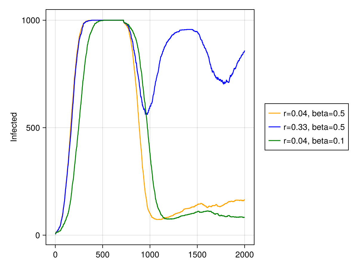
Exponential growth is evident in all cases.
Social distancing
Of course in reality a dampening mechanism will (hopefully) happen before all of the population is infected: a vaccine. This effectively introduces a 4th type of status, :V for vaccinated. This type can't get infected, and thus all remaining individuals that are already infected will (hopefully) survive or die out.
Until that point, social distancing is practiced. The best way to model social distancing is to make some agents simply not move (which feels like it approximates reality better).
sir_model = sir_initiation(isolated = 0.8)
abmvideo(
    "socialdist5.mp4",
    sir_model;
    title = "Social Distancing",
    frames = 100,
    spf = 2,
    ac = sir_colors,
    framerate = 20,
)
┌ Warning: keyword `spf` is deprecated in favor of `dt`.
└ @ AgentsVisualizations ~/.julia/packages/Agents/eKASH/ext/AgentsVisualizations/src/convenience.jl:102
┌ Warning: Keywords `as, am, ac` has been deprecated in favor of
│ `agent_size, agent_marker, agent_color`
└ @ AgentsVisualizations ~/.julia/packages/Agents/eKASH/ext/AgentsVisualizations/src/abmplot.jl:70Here we let some 20% of the population not be isolated, probably teenagers still partying, or anti-vaxers / flat-earthers that don't believe in science. Still, you can see that the spread of the virus is dramatically contained.
Let's look at the actual numbers, because animations are cool, but science is even cooler.
r4 = 0.04
sir_model4 = sir_initiation(reinfection_probability = r4, βmin = β1, isolated = 0.8)

data4, _ = run!(sir_model4, 2000; adata)

l4 = lines!(ax, data4[:, dataname((:status, infected))], color = :red)
figure[1, 2][2,1] = Legend(
    figure,
    [l4],
    ["r=$r4, social distancing"],
)
figure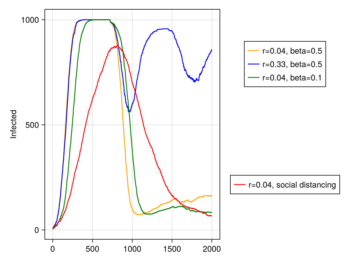
Here you can see the characteristic "flattening the curve" phrase you hear all over the news.