Wealth distribution model
This model is a simple agent-based economy that is modelled according to the work of Dragulescu et al.. This work introduces statistical mechanics concepts to study wealth distributions. What we show here is also referred to as "Boltzmann wealth distribution" model.
This model has a version with and without space. The rules of the space-less game are quite simple:
- There is a pre-determined number of agents.
- All agents start with one unit of wealth.
- At every step an agent gives 1 unit of wealth (if they have it) to some other agent.
Even though this rule-set is simple, it can still recreate the basic properties of wealth distributions, e.g. power-laws distributions.
Core structures: space-less
We start by defining the Agent type and initializing the model.
using Agents, Random

@agent struct WealthAgent(NoSpaceAgent)
    wealth::Int
end
Notice that this agent does not have a pos field. That is okay, because there is no space structure to this example. We can also make a very simple AgentBasedModel for our model.
function wealth_model(; numagents = 100, initwealth = 1, seed = 5)
    model = ABM(WealthAgent; agent_step!, scheduler = Schedulers.Randomly(),
                rng = Xoshiro(seed))
    for _ in 1:numagents
        add_agent!(model, initwealth)
    end
    return model
end
wealth_model (generic function with 1 method)The next step is to define the agent step function
function agent_step!(agent, model)
    agent.wealth == 0 && return # do nothing
    ragent = random_agent(model)
    agent.wealth -= 1
    ragent.wealth += 1
end

model = wealth_model()
StandardABM with 100 agents of type WealthAgent
agents container: Dict
space: nothing (no spatial structure)
scheduler: Agents.Schedulers.RandomlyWe use random_agent as a convenient way to just grab a second agent. (this may return the same agent as agent, but we don't care in the long run)
Running the space-less model
Let's do some data collection, running a large model for a lot of time
N = 5
M = 2000
adata = [:wealth]
model = wealth_model(numagents = M)
data, _ = run!(model, N; adata)
data[(end-20):end, :]| Row | time | id | wealth |
|---|---|---|---|
| Int64 | Int64 | Int64 | |
| 1 | 5 | 1980 | 0 |
| 2 | 5 | 1981 | 2 |
| 3 | 5 | 1982 | 1 |
| 4 | 5 | 1983 | 0 |
| 5 | 5 | 1984 | 1 |
| 6 | 5 | 1985 | 2 |
| 7 | 5 | 1986 | 0 |
| 8 | 5 | 1987 | 0 |
| 9 | 5 | 1988 | 0 |
| 10 | 5 | 1989 | 1 |
| 11 | 5 | 1990 | 0 |
| 12 | 5 | 1991 | 0 |
| 13 | 5 | 1992 | 0 |
| 14 | 5 | 1993 | 1 |
| 15 | 5 | 1994 | 0 |
| 16 | 5 | 1995 | 0 |
| 17 | 5 | 1996 | 0 |
| 18 | 5 | 1997 | 1 |
| 19 | 5 | 1998 | 0 |
| 20 | 5 | 1999 | 0 |
| 21 | 5 | 2000 | 4 |
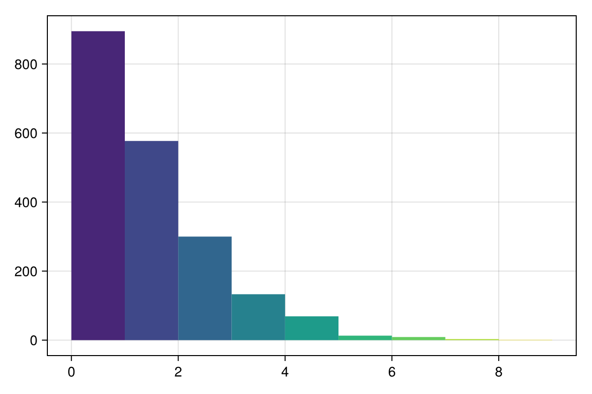
What we mostly care about is the distribution of wealth, which we can obtain for example by doing the following query:
wealths = filter(x -> x.time == N - 1, data)[!, :wealth]2000-element Vector{Int64}:
0
0
0
1
0
0
0
1
2
1
⋮
0
2
1
0
1
2
0
0
4and then we can make a histogram of the result. With a simple visualization we immediately see the power-law distribution:
using CairoMakie
hist(
    wealths;
    bins = collect(0:9),
    width = 1,
    color = cgrad(:viridis)[28:28:256],
    figure = (size = (600, 400),),
)
Core structures: with space
We now expand this model to (in this case) a 2D grid. The rules are the same but agents exchange wealth only with their neighbors.
It is also available from the Models module as Models.wealth_distribution.
We therefore have to add a pos field as the second field of the agents:
@agent struct WealthInSpace(GridAgent{2})
    wealth::Int
end

function wealth_model_2D(; dims = (25, 25), wealth = 1, M = 1000)
    space = GridSpace(dims, periodic = true)
    model = ABM(WealthInSpace, space; agent_step! = agent_step_2d!,
                scheduler = Schedulers.Randomly())
    for _ in 1:M # add agents in random positions
        add_agent!(model, wealth)
    end
    return model
end
wealth_model_2D (generic function with 1 method)The agent actions are a just a bit more complicated in this example. Now the agents can only give wealth to agents that exist on the same or neighboring positions (their "neighbors").
function agent_step_2d!(agent, model)
    agent.wealth == 0 && return # do nothing
    neighboring_positions = collect(nearby_positions(agent.pos, model))
    push!(neighboring_positions, agent.pos) # also consider current position
    rpos = rand(abmrng(model), neighboring_positions) # the position that we will exchange with
    available_ids = ids_in_position(rpos, model)
    if length(available_ids) > 0
        random_neighbor_agent = model[rand(abmrng(model), available_ids)]
        agent.wealth -= 1
        random_neighbor_agent.wealth += 1
    end
end

model2D = wealth_model_2D()
StandardABM with 1000 agents of type WealthInSpace
agents container: Dict
space: GridSpace with size (25, 25), metric=chebyshev, periodic=true
scheduler: Agents.Schedulers.RandomlyRunning the model with space
init_wealth = 4
model = wealth_model_2D(; wealth = init_wealth)
adata = [:wealth, :pos]
data, _ = run!(model, 10; adata = adata, when = [1, 5, 9])
data[(end-20):end, :]| Row | time | id | wealth | pos |
|---|---|---|---|---|
| Int64 | Int64 | Int64 | Tuple… | |
| 1 | 9 | 980 | 9 | (9, 9) |
| 2 | 9 | 981 | 1 | (21, 24) |
| 3 | 9 | 982 | 11 | (3, 11) |
| 4 | 9 | 983 | 0 | (2, 18) |
| 5 | 9 | 984 | 0 | (22, 5) |
| 6 | 9 | 985 | 10 | (10, 2) |
| 7 | 9 | 986 | 1 | (3, 23) |
| 8 | 9 | 987 | 1 | (9, 2) |
| 9 | 9 | 988 | 3 | (13, 12) |
| 10 | 9 | 989 | 6 | (23, 3) |
| 11 | 9 | 990 | 7 | (25, 3) |
| 12 | 9 | 991 | 0 | (16, 1) |
| 13 | 9 | 992 | 8 | (20, 21) |
| 14 | 9 | 993 | 3 | (17, 15) |
| 15 | 9 | 994 | 5 | (16, 19) |
| 16 | 9 | 995 | 3 | (15, 10) |
| 17 | 9 | 996 | 3 | (14, 10) |
| 18 | 9 | 997 | 0 | (20, 6) |
| 19 | 9 | 998 | 1 | (12, 2) |
| 20 | 9 | 999 | 4 | (13, 18) |
| 21 | 9 | 1000 | 4 | (17, 10) |
Okay, now we want to get the 2D spatial wealth distribution of the model. That is actually straightforward:
function wealth_distr(data, model, n)
    W = zeros(Int, size(abmspace(model)))
    for row in eachrow(filter(r -> r.time == n, data)) # iterate over rows at a specific step
        W[row.pos...] += row.wealth
    end
    return W
end

function make_heatmap(W)
    figure = Figure(; size = (600, 450))
    hmap_l = figure[1, 1] = Axis(figure)
    hmap = heatmap!(hmap_l, W; colormap = cgrad(:default))
    cbar = figure[1, 2] = Colorbar(figure, hmap; width = 30)
    return figure
end

W1 = wealth_distr(data, model2D, 1)
make_heatmap(W1)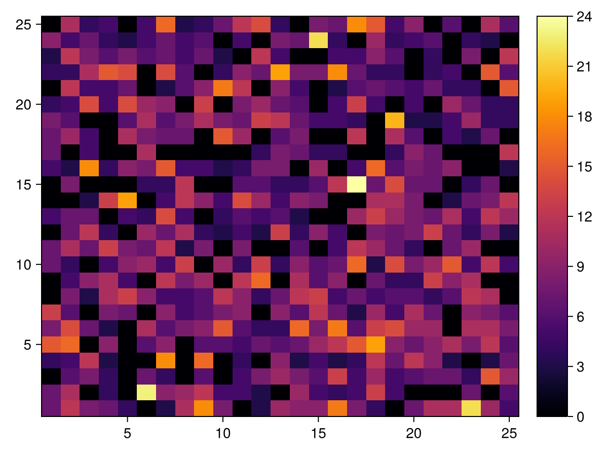
W5 = wealth_distr(data, model2D, 5)
make_heatmap(W5)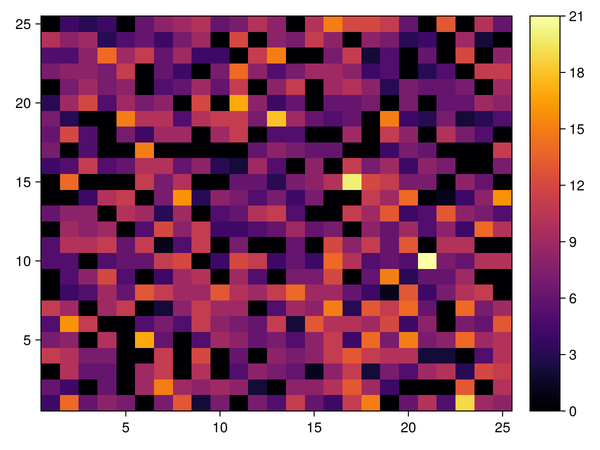
W10 = wealth_distr(data, model2D, 9)
make_heatmap(W10)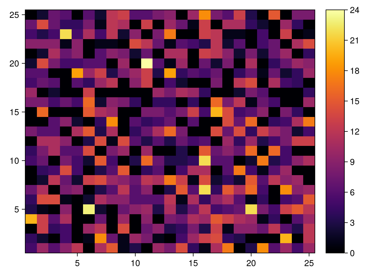
What we see is that wealth gets more and more localized.