Sugarscape
Growing Artificial Societies
(Descriptions below are from this page)
"Growing Artificial Societies" (Epstein & Axtell 1996) is a reference book for scientists interested in agent-based modelling and computer simulation. It represents one of the most paradigmatic and fascinating examples of the so-called generative approach to social science (Epstein 1999). In their book, Epstein & Axtell (1996) present a computational model where a heterogeneous population of autonomous agents compete for renewable resources that are unequally distributed over a 2-dimensional environment. Agents in the model are autonomous in that they are not governed by any central authority and they are heterogeneous in that they differ in their genetic attributes and their initial environmental endowments (e.g. their initial location and wealth). The model grows in complexity through the different chapters of the book as the agents are given the ability to engage in new activities such as sex, cultural exchange, trade, combat, disease transmission, etc. The core of Sugarscape has provided the basis for various extensions to study e.g. norm formation through cultural diffusion (Flentge et al. 2001) and the emergence of communication and cooperation in artificial societies (Buzing et al. 2005). Here we analyse the model described in the second chapter of Epstein & Axtell's (1996) book within the Markov chain framework.
Rules of sugarscape
The first model that Epstein & Axtell (1996) present comprises a finite population of agents who live in an environment. The environment is represented by a two-dimensional grid which contains sugar in some of its cells, hence the name Sugarscape. Agents' role in this first model consists in wandering around the Sugarscape harvesting the greatest amount of sugar they can find.
Environment
The environment is a 50×50 grid that wraps around forming a torus. Grid positions have both a sugar level and a sugar capacity c. A cell's sugar level is the number of units of sugar in the cell (potentially none), and its sugar capacity c is the maximum value the sugar level can take on that cell. Sugar capacity is fixed for each individual cell and may be different for different cells. The spatial distribution of sugar capacities depicts a sugar topography consisting of two peaks (with sugar capacity c = 4) separated by a valley, and surrounded by a desert region of sugarless cells (see Figure 1). Note, however, that the grid wraps around in both directions.
The Sugarscape obbeys the following rule:
Sugarscape growback rule G$\alpha$: At each position, sugar grows back at a rate of $\alpha$ units per time-step up to the cell's capacity c.
Agents
Every agent is endowed with individual (life-long) characteristics that condition her skills and capacities to survive in the Sugarscape. These individual attributes are:
- A vision v, which is the maximum number of positions the agent can see in each of
the four principal lattice directions: north, south, east and west.
- A metabolic rate m, which represents the units of sugar the agent burns per time-step.
- A maximum age max-age, which is the maximum number of time-steps the agent can live.
Agents also have the capacity to accumulate sugar wealth w. An agent's sugar wealth is incremented at the end of each time-step by the sugar collected and decremented by the agent's metabolic rate. Two agents are not allowed to occupy the same position in the grid.
The agents' behaviour is determined by the following two rules:
Agent movement rule M:
Consider the set of unoccupied positions within your vision (including the one you are standing on), identify the one(s) with the greatest amount of sugar, select the nearest one (Randomly() if there is more than one), move there and collect all the sugar in it. At this point, the agent's accumulated sugar wealth is incremented by the sugar collected and decremented by the agent's metabolic rate m. If at this moment the agent's sugar wealth is not greater than zero, then the agent dies.
Agent replacement rule R:
Whenever an agent dies it is replaced by a new agent of age 0 placed on a Randomly() chosen unoccupied position, having random attributes v, m and max-age, and random initial wealth w0. All random numbers are drawn from uniform distributions with ranges specified in Table 1 below.
Scheduling of events
Scheduling is determined by the order in which the different rules G, M and R are fired in the model. Environmental rule G comes first, followed by agent rule M (which is executed by all agents in random order) and finally agent rule R is executed (again, by all agents in random order).
Parameterisation
Our analysis corresponds to a model used by Epstein & Axtell (1996, pg. 33) to study the emergent wealth distribution in the agent population. This model is parameterised as indicated in Table 1 below (where U[a,b] denotes a uniform distribution with range [a,b]).
Initially, each position of the Sugarscape contains a sugar level equal to its sugar capacity c, and the 250 agents are created at a random unoccupied initial location and with random attributes (using the uniform distributions indicated in Table 1).
Table 1
| Parameter | Value |
|---|---|
| Lattice length L | 50 |
| Number of sugar peaks | 2 |
| Growth rate $\alpha$ | 1 |
| Number of agents N | 250 |
| Agents' initial wealth w0 distribution | U[5,25] |
| Agents' metabolic rate m distribution | U[1,4] |
| Agents' vision v distribution | U[1,6] |
| Agents' maximum age max-age distribution | U[60,100] |
Creating the ABM
using Agents, Random

@agent struct SugarSeeker(GridAgent{2})
    vision::Int
    metabolic_rate::Int
    age::Int
    max_age::Int
    wealth::Int
end
Functions distances and sugar_caps produce a matrix for the distribution of sugar capacities.
function distances(pos, sugar_peaks)
    all_dists = zeros(Int, length(sugar_peaks))
    for (ind, peak) in enumerate(sugar_peaks)
        d = round(Int, sqrt(sum((pos .- peak) .^ 2)))
        all_dists[ind] = d
    end
    return minimum(all_dists)
end

function sugar_caps(dims, sugar_peaks, max_sugar, dia = 4)
    sugar_capacities = zeros(Int, dims)
    for i in 1:dims[1], j in 1:dims[2]
        sugar_capacities[i, j] = distances((i, j), sugar_peaks)
    end
    for i in 1:dims[1]
        for j in 1:dims[2]
            sugar_capacities[i, j] = max(0, max_sugar - (sugar_capacities[i, j] ÷ dia))
        end
    end
    return sugar_capacities
end

"Create a sugarscape ABM"
function sugarscape(;
    dims = (50, 50),
    sugar_peaks = ((10, 40), (40, 10)),
    growth_rate = 1,
    N = 250,
    w0_dist = (5, 25),
    metabolic_rate_dist = (1, 4),
    vision_dist = (1, 6),
    max_age_dist = (60, 100),
    max_sugar = 4,
    seed = 42
)
    sugar_capacities = sugar_caps(dims, sugar_peaks, max_sugar, 6)
    sugar_values = deepcopy(sugar_capacities)
    space = GridSpaceSingle(dims)
    properties = Dict(
        :growth_rate => growth_rate,
        :N => N,
        :w0_dist => w0_dist,
        :metabolic_rate_dist => metabolic_rate_dist,
        :vision_dist => vision_dist,
        :max_age_dist => max_age_dist,
        :sugar_values => sugar_values,
        :sugar_capacities => sugar_capacities,
    )
    model = StandardABM(
        SugarSeeker,
        space;
        agent_step!,
        model_step!,
        scheduler = Schedulers.Randomly(),
        properties = properties,
        rng = MersenneTwister(seed)
    )
    for _ in 1:N
        add_agent_single!(
            model,
            rand(abmrng(model), vision_dist[1]:vision_dist[2]),
            rand(abmrng(model), metabolic_rate_dist[1]:metabolic_rate_dist[2]),
            0,
            rand(abmrng(model), max_age_dist[1]:max_age_dist[2]),
            rand(abmrng(model), w0_dist[1]:w0_dist[2]),
        )
    end
    return model
endMain.sugarscapeDefining stepping functions
Now we define the stepping functions that handle the time evolution of the model. The model stepping function controls the sugar growth:
function model_step!(model)
    # At each position, sugar grows back at a rate of α units
    # per time-step up to the cell's capacity c.
    @inbounds for pos in positions(model)
        if model.sugar_values[pos...] < model.sugar_capacities[pos...]
            model.sugar_values[pos...] += model.growth_rate
        end
    end
    return
end
model_step! (generic function with 1 method)The agent stepping function contains the dynamics of the model:
function agent_step!(agent, model)
    move_and_collect!(agent, model)
    replacement!(agent, model)
end

function move_and_collect!(agent, model)
    # Go through all unoccupied positions within vision, and consider the empty ones.
    # From those, identify the one with greatest amount of sugar, and go there!
    max_sugar_pos = agent.pos
    max_sugar = model.sugar_values[max_sugar_pos...]
    for pos in nearby_positions(agent, model, agent.vision)
        isempty(pos, model) || continue
        sugar = model.sugar_values[pos...]
        if sugar > max_sugar
            max_sugar = sugar
            max_sugar_pos = pos
        end
    end
    # Move to the max sugar position (which could be where we are already)
    move_agent!(agent, max_sugar_pos, model)
    # Collect the sugar there and update wealth (collected - consumed)
    agent.wealth += (model.sugar_values[max_sugar_pos...] - agent.metabolic_rate)
    model.sugar_values[max_sugar_pos...] = 0
    # age
    agent.age += 1
    return
end

function replacement!(agent, model)
    # If the agent's sugar wealth become zero or less, it dies
    if agent.wealth ≤ 0 || agent.age ≥ agent.max_age
        remove_agent!(agent, model)
        # Whenever an agent dies, a young one is added to a random empty position
        add_agent_single!(
            model,
            rand(abmrng(model), model.vision_dist[1]:model.vision_dist[2]),
            rand(abmrng(model), model.metabolic_rate_dist[1]:model.metabolic_rate_dist[2]),
            0,
            rand(abmrng(model), model.max_age_dist[1]:model.max_age_dist[2]),
            rand(abmrng(model), model.w0_dist[1]:model.w0_dist[2]),
        )
    end
end

model = sugarscape()
StandardABM with 250 agents of type SugarSeeker
agents container: Dict
space: GridSpaceSingle with size (50, 50), metric=chebyshev, periodic=true
scheduler: Agents.Schedulers.Randomly
properties: growth_rate, N, max_age_dist, metabolic_rate_dist, vision_dist, sugar_values, sugar_capacities, w0_distLet's plot the spatial distribution of sugar capacities in the Sugarscape.
using CairoMakie

fig = Figure(size = (600, 600))
ax, hm = heatmap(fig[1,1], model.sugar_capacities; colormap=:thermal)
Colorbar(fig[1, 2], hm, width = 20)
fig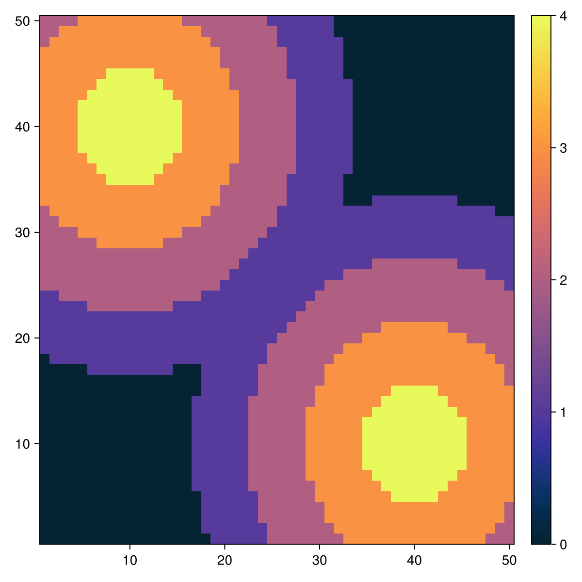
Plotting & Animating
We can plot the ABM and the sugar distribution side by side using abmplot and standard Makie.jl commands like lifting the model observable. (we could plot the sugar distribution as a heatmap, but we choose this composite plot for more variaty in the example pool)
model = sugarscape()
fig, ax, abmp = abmplot(model; add_controls = false, figkwargs = (size = (800, 600)))
# Lift model observable for heatmap
sugar = @lift($(abmp.model).sugar_values)
axhm, hm = heatmap(fig[1,2], sugar; colormap=:thermal, colorrange=(0,4))
axhm.aspect = AxisAspect(1) # equal aspect ratio for heatmap
Colorbar(fig[1, 3], hm, width = 15, tellheight=false)
rowsize!(fig.layout, 1, axhm.scene.px_area[].widths[2]) # Colorbar height = axis height
fig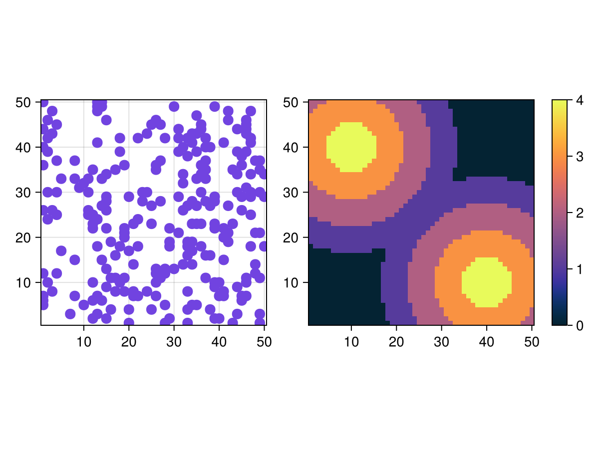
Animating this is now trivial. We simply step the model observable in abmp. We'll also add a title that counts the step number
s = Observable(0) # counter of current step, also observable
t = @lift("Sugarscape, step = $($(s))")
connect!(ax.title, t)
ax.titlealign = :left
fig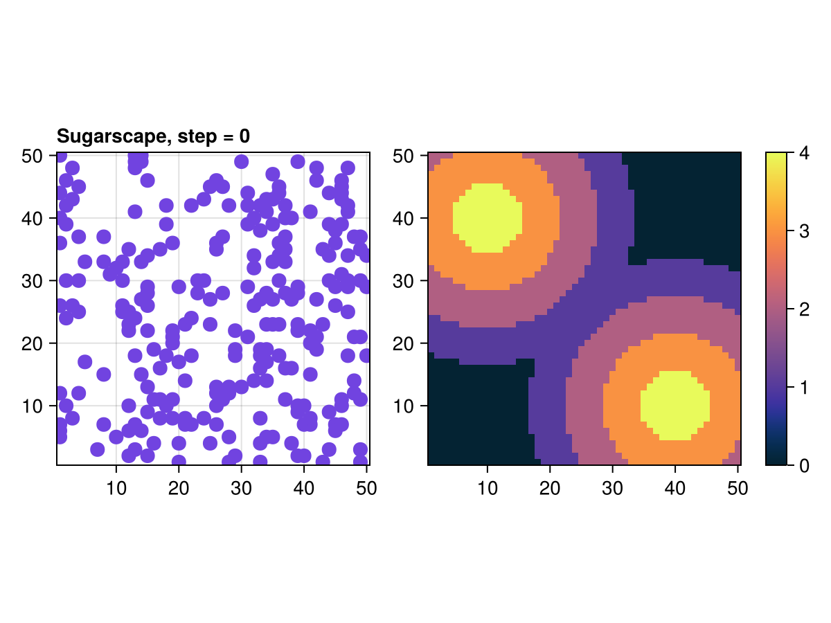
We animate the evolution of both the ABM and the sugar distribution using the following simple loop involving the abmstepper
record(fig, "sugarvis.mp4", 0:100; framerate = 3) do j
    # This updates the abm plot and lifted heatmap
    Agents.step!(abmp, 1)
    # This updates the title counter
    s[] = s[] + 1
end"sugarvis.mp4"Distribution of wealth across individuals
First we produce some data that include the wealth
model2 = sugarscape()
adata, _ = run!(model2, 100, adata = [:wealth])
adata[1:10,:]| Row | time | id | wealth |
|---|---|---|---|
| Int64 | Int64 | Int64 | |
| 1 | 0 | 1 | 18 |
| 2 | 0 | 2 | 9 |
| 3 | 0 | 3 | 24 |
| 4 | 0 | 4 | 6 |
| 5 | 0 | 5 | 21 |
| 6 | 0 | 6 | 20 |
| 7 | 0 | 7 | 18 |
| 8 | 0 | 8 | 11 |
| 9 | 0 | 9 | 20 |
| 10 | 0 | 10 | 12 |
And now we animate the evolution of the distribution of wealth
figure = Figure(size = (600, 600))
step_number = Observable(0)
title_text = @lift("Wealth distribution of individuals, step = $($step_number)")
Label(figure[1, 1], title_text; fontsize=20, tellwidth=false)
ax = Axis(figure[2, 1]; xlabel="Wealth", ylabel="Number of agents")
histdata = Observable(adata[adata.time .== 20, :wealth])
hist!(ax, histdata; bar_position=:time)
ylims!(ax, (0, 50))
record(figure, "sugarhist.mp4", 0:50; framerate=3) do i
    histdata[] = adata[adata.time .== i, :wealth]
    step_number[] = i
    xlims!(ax, (0, max(histdata[]...)))
end"sugarhist.mp4"We see that the distribution of wealth shifts from a more or less uniform distribution to a skewed distribution resembling a power-law.
References
BUZING P, Eiben A & Schut M (2005) Emerging communication and cooperation in evolving agent societies. Journal of Artificial Societies and Social Simulation 8(1)2. http://jasss.soc.surrey.ac.uk/8/1/2.html.
EPSTEIN J M (1999) Agent-Based Computational Models And Generative Social Science. Complexity 4(5), pp. 41-60.
EPSTEIN J M & Axtell R L (1996) Growing Artificial Societies: Social Science from the Bottom Up. The MIT Press.
FLENTGE F, Polani D & Uthmann T (2001) Modelling the emergence of possession norms using memes. Journal of Artificial Societies and Social Simulation 4(4)3. http://jasss.soc.surrey.ac.uk/4/4/3.html.