Spatial rock-paper-scissors (event based)

This is an introductory example. Similarly to Schelling's segregation model of the main Tutorial, its goal is to provide a tutorial for the EventQueueABM instead of the StandardABM. It assumes that you have gone through the Tutorial first.

The spatial rock-paper-scissors (RPS) is an ABM with the following rules:

• Agents can be any of three "kinds": Rock, Paper, or Scissors.
• Agents live in a 2D periodic grid space allowing only one agent per cell.
• When an agent activates, it can do one of three actions:
  1. Attack: choose a random nearby agent and attack it. If the agent loses the RPS game it gets removed.
  2. Move: choose a random nearby position. If it is empty move to it, otherwise swap positions with the agent there.
  3. Reproduce: choose a random empty nearby position (if any exist). Generate there a new agent of the same type.

And that's it really! However, we want to model this ABM as an event-based model. This means that these three actions are independent events that will get added to a queue of events. We will address this in a moment. For now, let's just make functions that represent the actions of the events.

Defining the event functions

We start by loading Agents

using Agents

and defining the three agent types using multiagent (see the main Tutorial if you are unfamiliar with @multiagent).

@multiagent struct RPS(GridAgent{2})
    @subagent struct Rock end
    @subagent struct Paper end
    @subagent struct Scissors end
end

Actions of events are standard Julia functions that utilize Agents.jl API, exactly like those given as agent_step! in StandardABM. They act on an agent and take the model as the second input and end with an empty return statement (as their return value is not utilized by Agents.jl).

The first action is the attack:

function attack!(agent, model)
    # Randomly pick a nearby agent
    contender = random_nearby_agent(agent, model)
    # do nothing if there isn't anyone nearby
    isnothing(contender) && return
    # else perform standard rock paper scissors logic
    # and remove the contender if you win.
    # Remember to compare agents with `kindof` instead of
    # `typeof` since we use `@multiagent` (see main Tutorial)
    kind = kindof(agent)
    kindc = kindof(contender)
    if kind === :Rock && kindc === :Scissors
        remove_agent!(contender, model)
    elseif kind === :Scissors && kindc === :Paper
        remove_agent!(contender, model)
    elseif kind === :Paper && kindc === :Rock
        remove_agent!(contender, model)
    end
    return
end

attack! (generic function with 1 method)

The movement function is equally simple due to the many functions offered by Agents.jl API.

function move!(agent, model)
    rand_pos = random_nearby_position(agent.pos, model)
    if isempty(rand_pos, model)
        move_agent!(agent, rand_pos, model)
    else
        occupant_id = id_in_position(rand_pos, model)
        occupant = model[occupant_id]
        swap_agents!(agent, occupant, model)
    end
    return
end

move! (generic function with 1 method)

The reproduction function is the simplest one.

function reproduce!(agent, model)
    pos = random_nearby_position(agent, model, 1, pos -> isempty(pos, model))
    isnothing(pos) && return
    # pass target position as a keyword argument
    replicate!(agent, model; pos)
    return
end

# Defining the propensity and timing of the events

reproduce! (generic function with 1 method)

Besides the actual event action defined as the above functions, there are two more pieces of information necessary:

1. how likely an event is to happen, and
2. how long after the previous event it will happen.

Now, in the "Gillespie" type of simulations, these two things coincide: The probability for an event is its relative propensity (rate), and the time you have to wait for it to happen is inversely the propensity (rate). When creating an AgentEvent (see below), the user has the option to go along this "Gillespie" route, which is the default. However, the user can also have more control by explicitly providing a function that returns the time until an event triggers (by default this function becomes a random sample of an exponential distribution).

Let's make this concrete. For all events we need to define their propensities. Another way to think of propensities is the relative probability mass for an event to happen. The propensities may be constants or functions of the currently actived agent and the model.

Here, the propensities for moving and attacking will be constants,

attack_propensity = 1.0
movement_propensity = 0.5

0.5

while the propensity for reproduction will be a function modelling "seasonality", so that willingness to reproduce goes up and down periodically

function reproduction_propensity(agent, model)
    return cos(abmtime(model))^2
end

# Creating the `AgentEvent` structures

reproduction_propensity (generic function with 1 method)

Events are registered as an AgentEvent, then are added into a container, and then given to the EventQueueABM. The attack and reproduction events affect all agents, and hence we don't need to specify what agents they apply to.

attack_event = AgentEvent(action! = attack!, propensity = attack_propensity)

reproduction_event = AgentEvent(action! = reproduce!, propensity = reproduction_propensity)

AgentEvent{typeof(Main.reproduce!), typeof(Main.reproduction_propensity), Nothing, typeof(Agents.exp_propensity)}(Main.reproduce!, Main.reproduction_propensity, nothing, Agents.exp_propensity)

The movement event does not apply to rocks however, so we need to specify the agent "kinds" that it applies to, which is (:Scissors, :Paper). Additionally, we would like to change how the timing of the movement events works. We want to change it from an exponential distribution sample to something else. This "something else" is once again an arbitrary Julia function, and for here we will make:

function movement_time(agent, model, propensity)
    # `agent` is the agent the event will be applied to,
    # which we do not use in this function!
    t = 0.1 * randn(abmrng(model)) + 1
    return clamp(t, 0, Inf)
end

movement_time (generic function with 1 method)

And with this we can now create

movement_event = AgentEvent(
    action! = move!, propensity = movement_propensity,
    kinds = (:Scissors, :Paper), timing = movement_time
)

AgentEvent{typeof(Main.move!), Float64, Tuple{Symbol, Symbol}, typeof(Main.movement_time)}(Main.move!, 0.5, (:Scissors, :Paper), Main.movement_time)

we wrap all events in a tuple and we are done with the setting up part!

events = (attack_event, reproduction_event, movement_event)

(AgentEvent{typeof(Main.attack!), Float64, Nothing, typeof(Agents.exp_propensity)}(Main.attack!, 1.0, nothing, Agents.exp_propensity), AgentEvent{typeof(Main.reproduce!), typeof(Main.reproduction_propensity), Nothing, typeof(Agents.exp_propensity)}(Main.reproduce!, Main.reproduction_propensity, nothing, Agents.exp_propensity), AgentEvent{typeof(Main.move!), Float64, Tuple{Symbol, Symbol}, typeof(Main.movement_time)}(Main.move!, 0.5, (:Scissors, :Paper), Main.movement_time))

Creating and populating the EventQueueABM

This step is almost identical to making a StandardABM in the main Tutorial. We create an instance of EventQueueABM by giving it the agent type it will have, the events, and a space (optionally, defaults to no space). Here we have

space = GridSpaceSingle((100, 100))

using Random: Xoshiro
rng = Xoshiro(42)

model = EventQueueABM(RPS, events, space; rng, warn = false)

EventQueueABM{GridSpaceSingle{2, true}, Main.RPS, Dict{Int64, Main.RPS}, Nothing, Tuple{AgentEvent{typeof(Main.attack!), Float64, Nothing, typeof(Agents.exp_propensity)}, AgentEvent{typeof(Main.reproduce!), typeof(Main.reproduction_propensity), Nothing, typeof(Agents.exp_propensity)}, AgentEvent{typeof(Main.move!), Float64, Tuple{Symbol, Symbol}, typeof(Main.movement_time)}}, Random.Xoshiro, Vector{Vector{Int64}}, Vector{Vector{Float64}}, Vector{Vector{Int64}}, DataStructures.BinaryHeap{Pair{Tuple{Int64, Int64}, Float64}, Base.Order.By{typeof(last), Base.Order.ForwardOrdering}}}(Dict{Int64, Main.RPS}(), GridSpaceSingle with size (100, 100), metric=chebyshev, periodic=true, nothing, Random.Xoshiro(0xa379de7eeeb2a4e8, 0x953dccb6b532b3af, 0xf597b8ff8cfd652a, 0xccd7337c571680d1, 0xc90c4a0730db3f7e), Base.RefValue{Int64}(0), Base.RefValue{Float64}(0.0), (AgentEvent{typeof(Main.attack!), Float64, Nothing, typeof(Agents.exp_propensity)}(Main.attack!, 1.0, nothing, Agents.exp_propensity), AgentEvent{typeof(Main.reproduce!), typeof(Main.reproduction_propensity), Nothing, typeof(Agents.exp_propensity)}(Main.reproduce!, Main.reproduction_propensity, nothing, Agents.exp_propensity), AgentEvent{typeof(Main.move!), Float64, Tuple{Symbol, Symbol}, typeof(Main.movement_time)}(Main.move!, 0.5, (:Scissors, :Paper), Main.movement_time)), Dict(:Paper => 2, :Rock => 1, :Scissors => 3), [[1, 2], [1, 2, 3], [1, 2, 3]], [[1.0, 0.0], [1.0, 0.0, 0.5], [1.0, 0.0, 0.5]], [[2], [2], [2]], DataStructures.BinaryHeap{Pair{Tuple{Int64, Int64}, Float64}, Base.Order.By{typeof(last), Base.Order.ForwardOrdering}}(Base.Order.By{typeof(last), Base.Order.ForwardOrdering}(last, Base.Order.ForwardOrdering()), Pair{Tuple{Int64, Int64}, Float64}[]), true, true)

populating the model with agents is the same as in the main Tutorial, using the add_agent! function. By default, when an agent is added to the model an event is also generated for it and added to the queue.

for p in positions(model)
    type = rand(abmrng(model), (Rock, Paper, Scissors))
    add_agent!(p, type, model)
end

We can see the list of scheduled events via

abmqueue(model)

DataStructures.BinaryHeap{Pair{Tuple{Int64, Int64}, Float64}, Base.Order.By{typeof(last), Base.Order.ForwardOrdering}}(Base.Order.By{typeof(last), Base.Order.ForwardOrdering}(last, Base.Order.ForwardOrdering()), [(6080, 1) => 2.9790681020079457e-6, (3987, 1) => 0.0003364593569030146, (6221, 2) => 0.0004887948187761659, (8424, 1) => 0.0006778319693496694, (5035, 1) => 0.0012044922191219774, (7014, 2) => 0.0005771225059120387, (3301, 2) => 0.0011396494447446436, (2505, 1) => 0.0014309955844005063, (5041, 2) => 0.001449028423933035, (5539, 2) => 0.0024520873429744127  …  (9990, 1) => 1.0666363792018059, (9992, 2) => 0.7429399475482082, (9993, 1) => 1.9378465659189394, (4997, 1) => 1.7907183401427267, (2496, 1) => 0.5304394096759053, (2499, 1) => 2.7442278746073216, (4998, 3) => 1.0804360033507288, (4999, 1) => 5.80807081086072, (9998, 1) => 0.9433255253597445, (1250, 3) => 1.258669914970242])

Here the queue maps pairs of (agent id, event index) to the time the events will trigger. There are currently as many scheduled events because as the amount of agents we added to the model. Note that the timing of the events has been rounded for display reasons!

Now, as per-usual in Agents.jl we are making a keyword-based function for constructing the model, so that it is easier to handle later.

function initialize_rps(; n = 100, nx = n, ny = n, seed = 42)
    space = GridSpaceSingle((nx, ny))
    rng = Xoshiro(seed)
    model = EventQueueABM(RPS, events, space; rng, warn = false)
    for p in positions(model)
        type = rand(abmrng(model), (Rock, Paper, Scissors))
        add_agent!(p, type, model)
    end
    return model
end

initialize_rps (generic function with 1 method)

Time evolution

Time evolution for EventBasedABM is identical to that of StandardABM, but time is continuous. So, when calling step! we pass in a real time.

step!(model, 123.456)

nagents(model)

9760

Alternatively we could give a function for when to terminate the time evolution. For example, we terminate if any of the three types of agents become less than a threshold

function terminate(model, t)
    kinds = allkinds(RPS)
    threshold = 1000
    # Alright, this code snippet loops over all kinds,
    # and for each it checks if it is less than the threshold.
    # if any is, it returns `true`, otherwise `false.`
    logic = any(kinds) do kind
        n = count(a -> kindof(a) == kind, allagents(model))
        return n < threshold
    end
    # For safety, in case this never happens, we also add a trigger
    # regarding the total evolution time
    return logic || (t > 1000.0)
end

step!(model, terminate)

abmtime(model)

139.84392719607195

Data collection

The entirety of the Agents.jl API is orthogonal/agnostic to what model we have. This means that whatever we do, plotting, data collection, etc., has identical syntax irrespectively of whether we have a StandardABM or EventQueueABM.

Hence, data collection also works almost identically to StandardABM.

Here we will simply collect the number of each agent kind.

model = initialize_rps()

adata = [(a -> kindof(a) === X, count) for X in allkinds(RPS)]

adf, mdf = run!(model, 100.0; adata, when = 0.5, dt = 0.01)

adf[1:10, :]

Let's visualize the population sizes versus time:

using Agents.DataFrames
using CairoMakie

tvec = adf[!, :time]
populations = adf[:, Not(:time)]
alabels = ["rocks", "papers", "scissors"]

fig = Figure();
ax = Axis(fig[1,1]; xlabel = "time", ylabel = "population")
for (i, l) in enumerate(alabels)
    lines!(ax, tvec, populations[!, i]; label = l)
end
axislegend(ax)
fig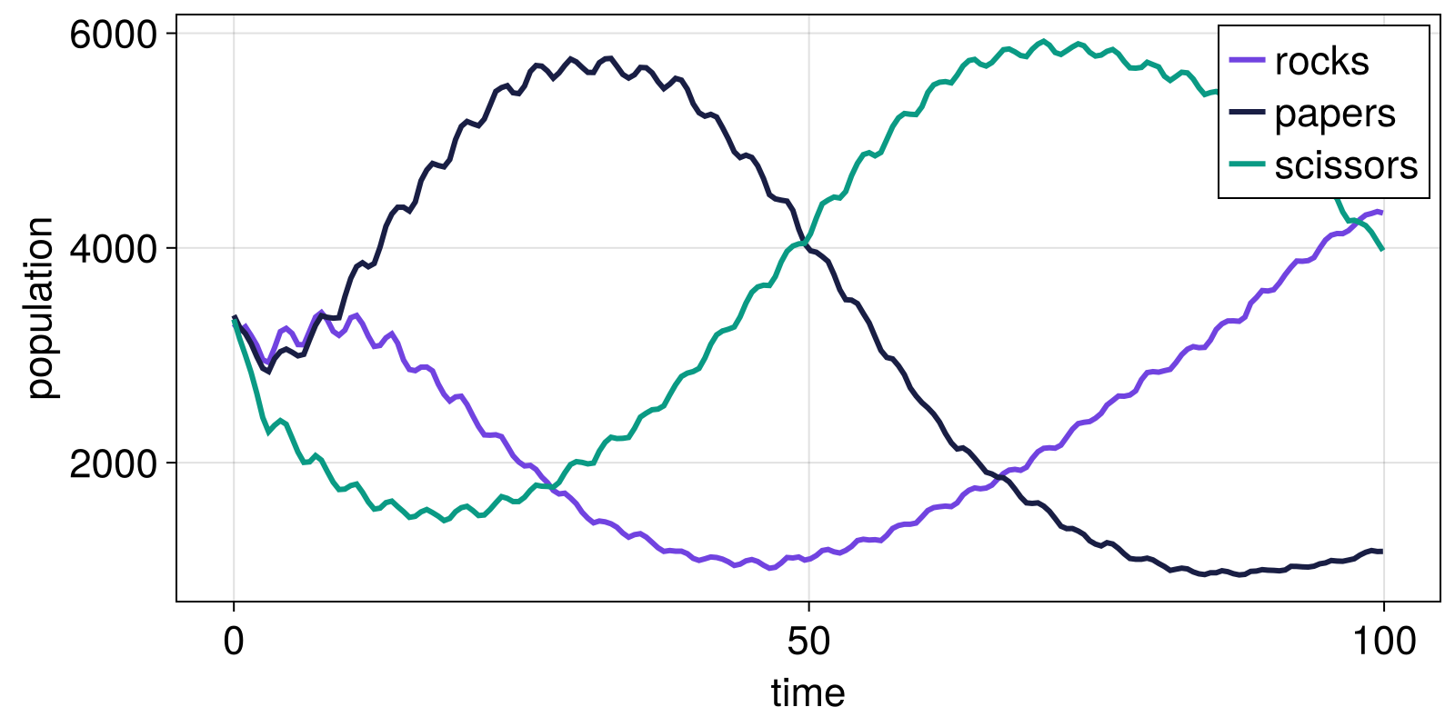

Visualization

Visualization for EventQueueABM is identical to that for StandardABM that we learned in the visualization tutorial. Naturally, for EventQueueABM the dt argument of abmvideo corresponds to continuous time and does not have to be an integer.

const colormap = Dict(:Rock => "black", :Scissors => "gray", :Paper => "orange")
agent_color(agent) = colormap[kindof(agent)]
plotkw = (agent_color, agent_marker = :rect, agent_size = 5)
fig, ax, abmobs = abmplot(model; plotkw...)

fig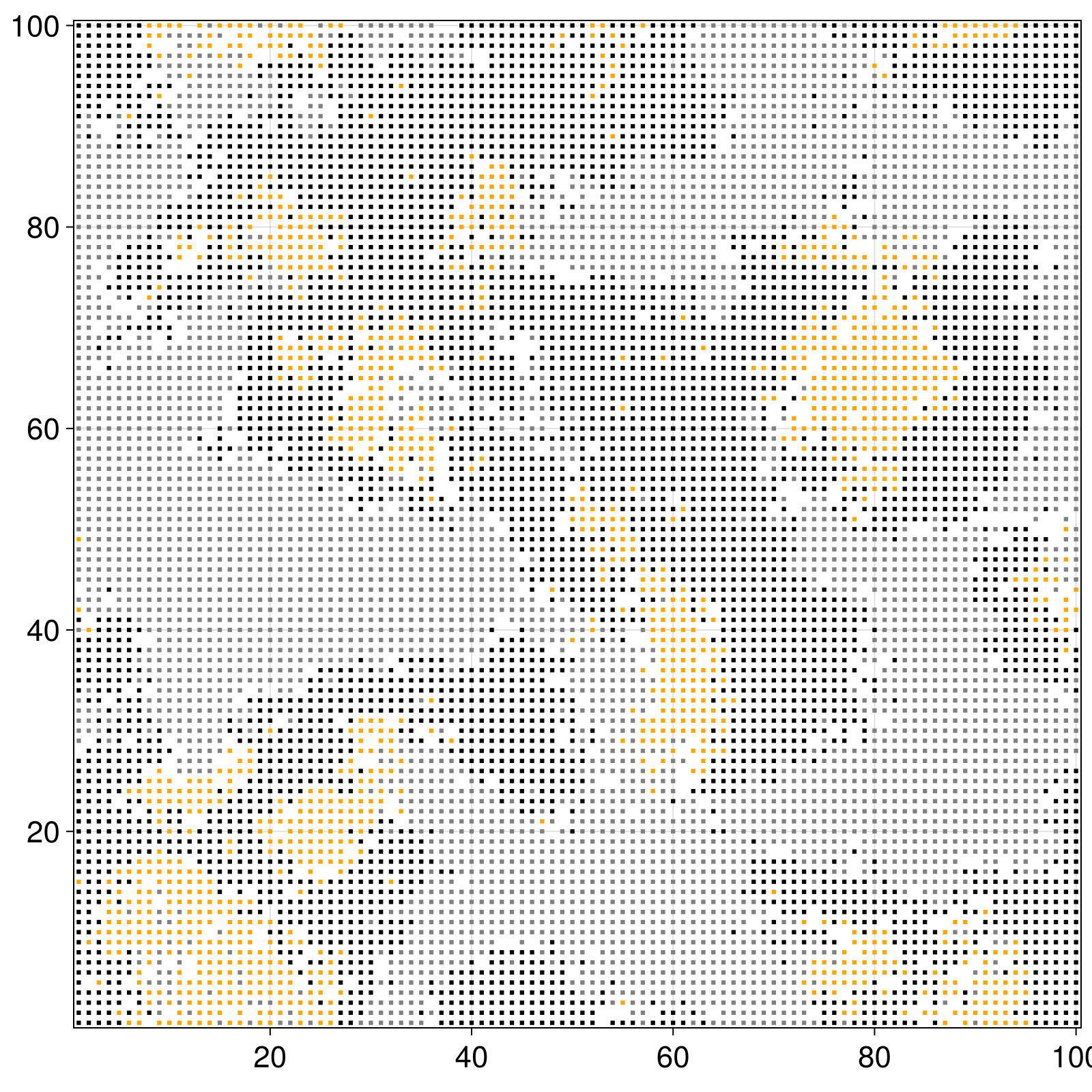

model = initialize_rps()
abmvideo("rps_eventqueue.mp4", model;
    dt = 0.5, frames = 300,
    title = "Rock Paper Scissors (event based)", plotkw...,
)

We see model dynamics similar to Schelling's segregation model: neighborhoods for same-type agents form! But they are not static, but rather expand and contract over time!

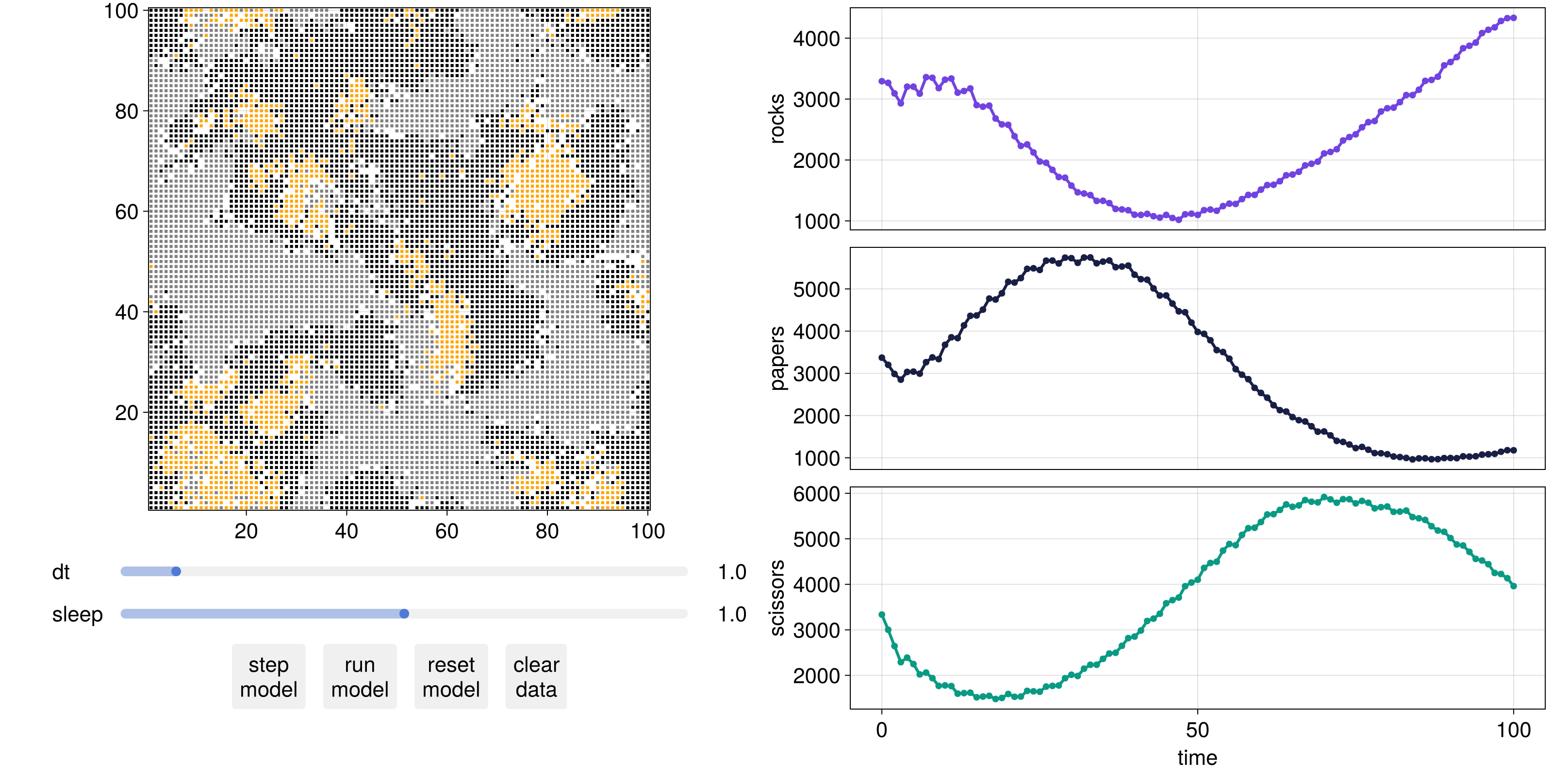
We could explore this interactively by launching the interactive GUI with the abmexploration function!

Let's first define the data we want to visualize, which in this case is just the count of each agent kind

model = initialize_rps()
fig, abmobs = abmexploration(model; adata, alabels, when = 0.5, plotkw...)
fig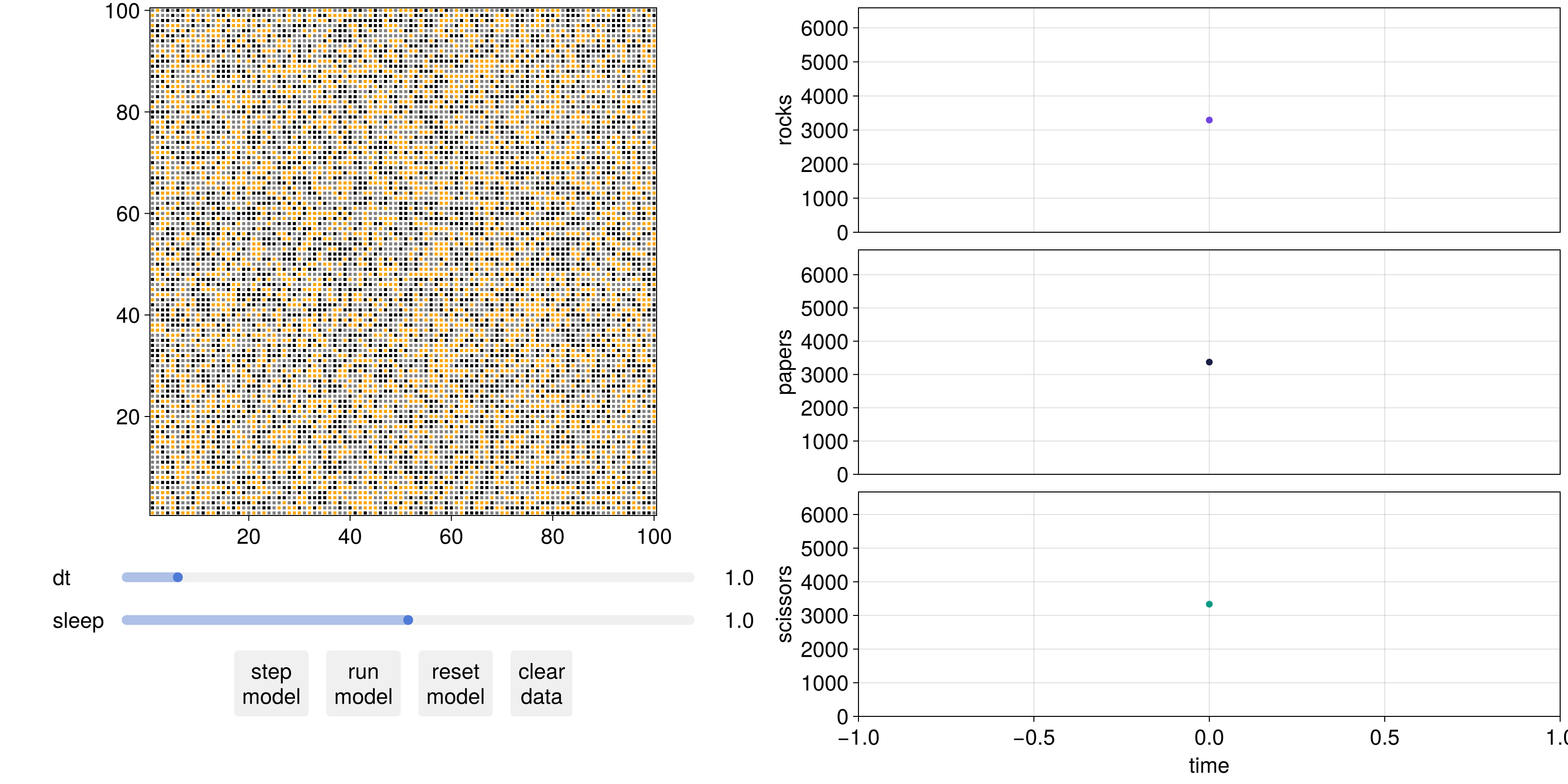

We can then step the observable and see the updates in the plot:

for _ in 1:100 # this loop simulates pressing the `run!` button
    step!(abmobs, 1.0)
end

fig