Predator-prey dynamics
The predator-prey model emulates the population dynamics of predator and prey animals who live in a common ecosystem and compete over limited resources. This model is an agent-based analog to the classic Lotka-Volterra differential equation model.
This example illustrates how to develop models with heterogeneous agents (sometimes referred to as a mixed agent based model), incorporation of a spatial property in the dynamics (represented by a standard array, not an agent, as is done in most other ABM frameworks), and usage of GridSpace, which allows multiple agents per grid coordinate.
Model specification
The environment is a two dimensional grid containing sheep, wolves and grass. In the model, wolves eat sheep and sheep eat grass. Their populations will oscillate over time if the correct balance of resources is achieved. Without this balance however, a population may become extinct. For example, if wolf population becomes too large, they will deplete the sheep and subsequently die of starvation.
We will begin by loading the required packages and defining two subtypes of AbstractAgent: Sheep, Wolf. Grass will be a spatial property in the model. All three agent types have id and pos properties, which is a requirement for all subtypes of AbstractAgent when they exist upon a GridSpace. Sheep and wolves have identical properties, but different behaviors as explained below. The property energy represents an animals current energy level. If the level drops below zero, the agent will die. Sheep and wolves reproduce asexually in this model, with a probability given by reproduction_prob. The property Δenergy controls how much energy is acquired after consuming a food source.
Grass is a replenishing resource that occupies every position in the grid space. Grass can be consumed only if it is fully_grown. Once the grass has been consumed, it replenishes after a delay specified by the property regrowth_time. The property countdown tracks the delay between being consumed and the regrowth time.
Making the model
First we define the agent types (here you can see that it isn't really that much of an advantage to have two different agent types. Like in the Rabbit, Fox, Hawk example, we could have only one type and one additional field to separate them. Nevertheless, for the sake of example, we will use two different types.)
using Agents, Random

@agent struct Sheep(GridAgent{2})
    energy::Float64
    reproduction_prob::Float64
    Δenergy::Float64
end

@agent struct Wolf(GridAgent{2})
    energy::Float64
    reproduction_prob::Float64
    Δenergy::Float64
end
The function initialize_model returns a new model containing sheep, wolves, and grass using a set of pre-defined values (which can be overwritten). The environment is a two dimensional grid space, which enables animals to walk in all directions.
function initialize_model(;
        n_sheep = 100,
        n_wolves = 50,
        dims = (20, 20),
        regrowth_time = 30,
        Δenergy_sheep = 4,
        Δenergy_wolf = 20,
        sheep_reproduce = 0.04,
        wolf_reproduce = 0.05,
        seed = 23182,
    )

    rng = MersenneTwister(seed)
    space = GridSpace(dims, periodic = true)
    # Model properties contain the grass as two arrays: whether it is fully grown
    # and the time to regrow. Also have static parameter `regrowth_time`.
    # Notice how the properties are a `NamedTuple` to ensure type stability.
    properties = (
        fully_grown = falses(dims),
        countdown = zeros(Int, dims),
        regrowth_time = regrowth_time,
    )
    model = StandardABM(
        Union{Sheep, Wolf}, space;
        agent_step! = sheepwolf_step!, model_step! = grass_step!,
        properties, rng, scheduler = Schedulers.Randomly(), warn = false
    )
    # Add agents
    for _ in 1:n_sheep
        energy = rand(abmrng(model), 1:(Δenergy_sheep * 2)) - 1
        add_agent!(Sheep, model, energy, sheep_reproduce, Δenergy_sheep)
    end
    for _ in 1:n_wolves
        energy = rand(abmrng(model), 1:(Δenergy_wolf * 2)) - 1
        add_agent!(Wolf, model, energy, wolf_reproduce, Δenergy_wolf)
    end
    # Add grass with random initial growth
    for p in positions(model)
        fully_grown = rand(abmrng(model), Bool)
        countdown = fully_grown ? regrowth_time : rand(abmrng(model), 1:regrowth_time) - 1
        model.countdown[p...] = countdown
        model.fully_grown[p...] = fully_grown
    end
    return model
end
initialize_model (generic function with 1 method)Defining the stepping functions
Sheep and wolves behave similarly: both lose 1 energy unit by moving to an adjacent position and both consume a food source if available. If their energy level is below zero, they die. Otherwise, they live and reproduce with some probability. They move to a random adjacent position with the randomwalk! function.
Notice how the function sheepwolf_step!, which is our agent_step!, is dispatched to the appropriate agent type via Julia's Multiple Dispatch system.
function sheepwolf_step!(sheep::Sheep, model)
    randomwalk!(sheep, model)
    sheep.energy -= 1
    if sheep.energy < 0
        remove_agent!(sheep, model)
        return
    end
    eat!(sheep, model)
    return if rand(abmrng(model)) ≤ sheep.reproduction_prob
        sheep.energy /= 2
        replicate!(sheep, model)
    end
end

function sheepwolf_step!(wolf::Wolf, model)
    randomwalk!(wolf, model; ifempty = false)
    wolf.energy -= 1
    if wolf.energy < 0
        remove_agent!(wolf, model)
        return
    end
    # If there is any sheep on this grid cell, it's dinner time!
    dinner = first_sheep_in_position(wolf.pos, model)
    !isnothing(dinner) && eat!(wolf, dinner, model)
    return if rand(abmrng(model)) ≤ wolf.reproduction_prob
        wolf.energy /= 2
        replicate!(wolf, model)
    end
end

function first_sheep_in_position(pos, model)
    ids = ids_in_position(pos, model)
    j = findfirst(id -> model[id] isa Sheep, ids)
    return isnothing(j) ? nothing : model[ids[j]]::Sheep
end
first_sheep_in_position (generic function with 1 method)Sheep and wolves have separate eat! functions. If a sheep eats grass, it will acquire additional energy and the grass will not be available for consumption until regrowth time has elapsed. If a wolf eats a sheep, the sheep dies and the wolf acquires more energy.
function eat!(sheep::Sheep, model)
    if model.fully_grown[sheep.pos...]
        sheep.energy += sheep.Δenergy
        model.fully_grown[sheep.pos...] = false
    end
    return
end

function eat!(wolf::Wolf, sheep::Sheep, model)
    remove_agent!(sheep, model)
    wolf.energy += wolf.Δenergy
    return
end
eat! (generic function with 2 methods)The behavior of grass function differently. If it is fully grown, it is consumable. Otherwise, it cannot be consumed until it regrows after a delay specified by regrowth_time. The dynamics of the grass is our model_step! function.
function grass_step!(model)
    return @inbounds for p in positions(model) # we don't have to enable bound checking
        if !(model.fully_grown[p...])
            if model.countdown[p...] ≤ 0
                model.fully_grown[p...] = true
                model.countdown[p...] = model.regrowth_time
            else
                model.countdown[p...] -= 1
            end
        end
    end
end

sheepwolfgrass = initialize_model()
StandardABM with 150 agents of type Union{Main.Sheep, Main.Wolf}
agents container: Dict
space: GridSpace with size (20, 20), metric=chebyshev, periodic=true
scheduler: Agents.Schedulers.Randomly
properties: fully_grown, countdown, regrowth_timeRunning the model
We will run the model for 500 steps and record the number of sheep, wolves and consumable grass patches after each step. First: initialize the model.
using CairoMakieTo view our starting population, we can build an overview plot using abmplot. We define the plotting details for the wolves and sheep:
offset(a) = a isa Sheep ? (-0.1, -0.1 * rand()) : (+0.1, +0.1 * rand())
ashape(a) = a isa Sheep ? :circle : :utriangle
acolor(a) = a isa Sheep ? RGBAf(1.0, 1.0, 1.0, 0.8) : RGBAf(0.2, 0.2, 0.3, 0.8)
acolor (generic function with 1 method)and instruct abmplot how to plot grass as a heatmap:
grasscolor(model) = model.countdown ./ model.regrowth_timegrasscolor (generic function with 1 method)and finally define a colormap for the grass:
heatkwargs = (colormap = [:brown, :green], colorrange = (0, 1))(colormap = [:brown, :green], colorrange = (0, 1))and put everything together and give it to abmplot
plotkwargs = (;
    agent_color = acolor,
    agent_size = 25,
    agent_marker = ashape,
    offset,
    agentsplotkwargs = (strokewidth = 1.0, strokecolor = :black),
    heatarray = grasscolor,
    heatkwargs = heatkwargs,
)

sheepwolfgrass = initialize_model()

fig, ax, abmobs = abmplot(sheepwolfgrass; plotkwargs...)
fig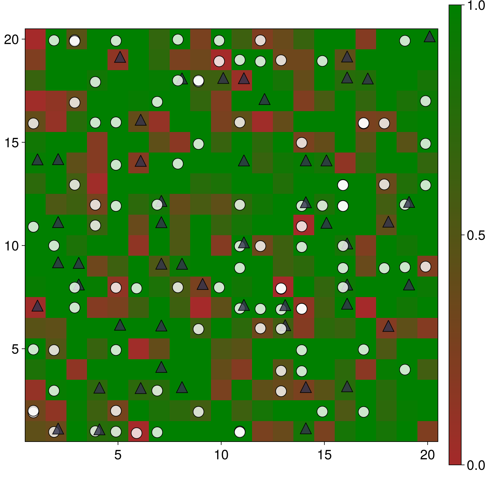
Now, lets run the simulation and collect some data. Define datacollection:
sheep(a) = a isa Sheep
wolf(a) = a isa Wolf
count_grass(model) = count(model.fully_grown)
count_grass (generic function with 1 method)Run simulation:
sheepwolfgrass = initialize_model()
steps = 1000
adata = [(sheep, count), (wolf, count)]
mdata = [count_grass]
adf, mdf = run!(sheepwolfgrass, steps; adata, mdata)(1001×3 DataFrame
Row │ time count_sheep count_wolf
│ Int64 Int64 Int64
──────┼────────────────────────────────
1 │ 0 100 50
2 │ 1 89 49
3 │ 2 76 50
4 │ 3 71 51
5 │ 4 64 51
6 │ 5 54 51
7 │ 6 48 52
8 │ 7 39 53
⋮ │ ⋮ ⋮ ⋮
995 │ 994 0 0
996 │ 995 0 0
997 │ 996 0 0
998 │ 997 0 0
999 │ 998 0 0
1000 │ 999 0 0
1001 │ 1000 0 0
986 rows omitted, 1001×2 DataFrame
Row │ time count_grass
│ Int64 Int64
──────┼────────────────────
1 │ 0 195
2 │ 1 163
3 │ 2 148
4 │ 3 129
5 │ 4 119
6 │ 5 115
7 │ 6 108
8 │ 7 112
⋮ │ ⋮ ⋮
995 │ 994 400
996 │ 995 400
997 │ 996 400
998 │ 997 400
999 │ 998 400
1000 │ 999 400
1001 │ 1000 400
986 rows omitted)The following plot shows the population dynamics over time. Initially, wolves become extinct because they consume the sheep too quickly. The few remaining sheep reproduce and gradually reach an equilibrium that can be supported by the amount of available grass.
function plot_population_timeseries(adf, mdf)
    figure = Figure(size = (600, 400))
    ax = figure[1, 1] = Axis(figure; xlabel = "Step", ylabel = "Population")
    sheepl = lines!(ax, adf.time, adf.count_sheep, color = :cornsilk4)
    wolfl = lines!(ax, adf.time, adf.count_wolf, color = RGBAf(0.2, 0.2, 0.3))
    grassl = lines!(ax, mdf.time, mdf.count_grass, color = :green)
    figure[1, 2] = Legend(figure, [sheepl, wolfl, grassl], ["Sheep", "Wolves", "Grass"])
    return figure
end

plot_population_timeseries(adf, mdf)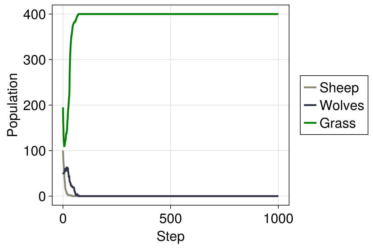
Altering the input conditions, we now see a landscape where sheep, wolves and grass find an equilibrium
stable_params = (;
    n_sheep = 140,
    n_wolves = 20,
    dims = (30, 30),
    Δenergy_sheep = 5,
    sheep_reproduce = 0.31,
    wolf_reproduce = 0.06,
    Δenergy_wolf = 30,
    seed = 71758,
)

sheepwolfgrass = initialize_model(; stable_params...)
adf, mdf = run!(sheepwolfgrass, 2000; adata, mdata)
plot_population_timeseries(adf, mdf)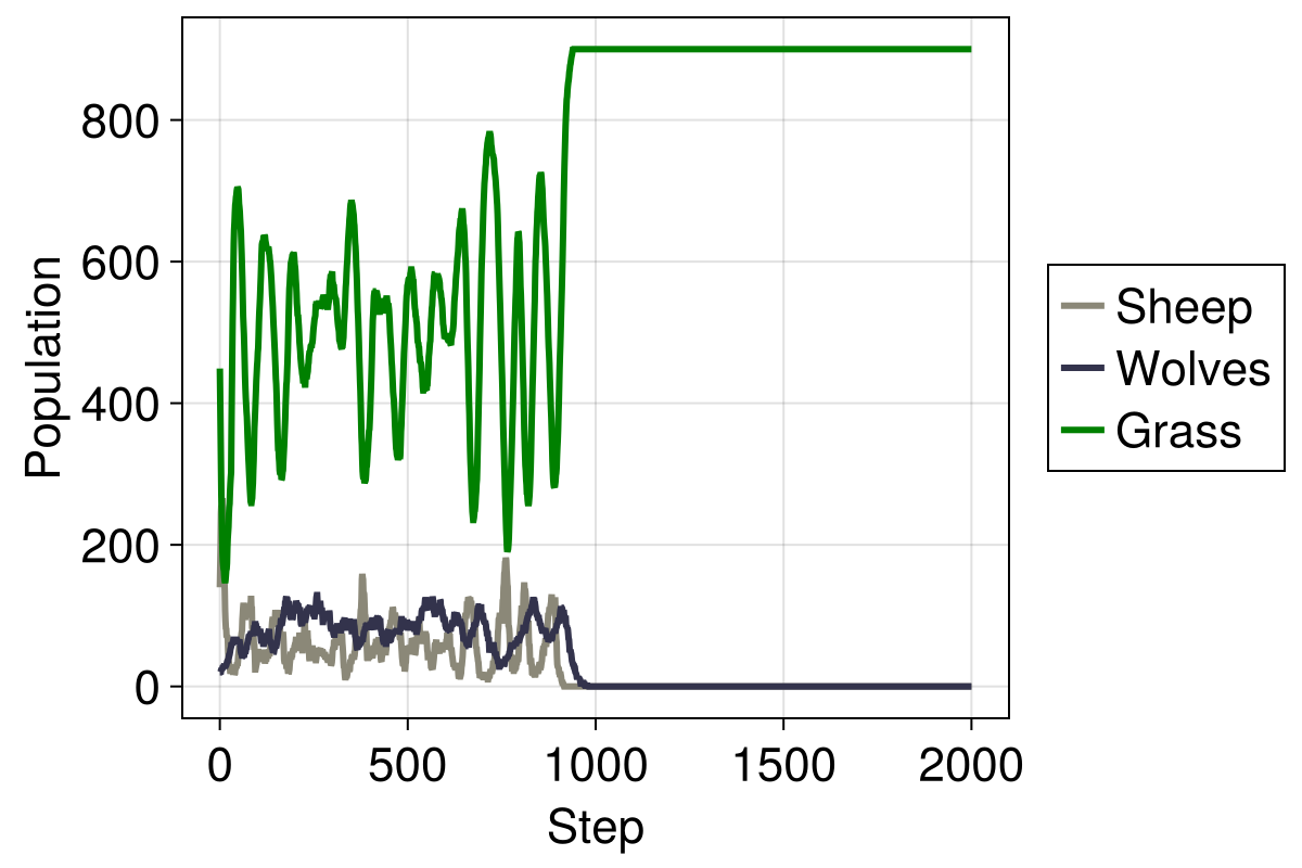
Finding a parameter combination that leads to long-term coexistence was surprisingly difficult. It is for such cases that the Optimizing agent based models example is useful!
Video
Given that we have defined plotting functions, making a video is as simple as
sheepwolfgrass = initialize_model(; stable_params...)

abmvideo(
    "sheepwolf.mp4",
    sheepwolfgrass;
    frames = 100,
    framerate = 8,
    title = "Sheep Wolf Grass",
    plotkwargs...,
)