Visualizations and Animations for Agent Based Models
This page describes functions that can be used with the Makie plotting ecosystem to animate and interact with agent based models. All the functionality described here uses Julia's package extensions and therefore comes into scope once Makie (or any of its backends such as CairoMakie) gets loaded.
The animation at the start of the page is created using the code of this page, see below.
The docs are built using versions:
import Pkg
Pkg.status(
    ["Agents", "CairoMakie"];
    mode = Pkg.PKGMODE_MANIFEST, io = stdout
)
Status `~/work/Agents.jl/Agents.jl/docs/Manifest.toml`
[46ada45e] Agents v7.0.3 `~/work/Agents.jl/Agents.jl`
⌃ [13f3f980] CairoMakie v0.13.10
Info Packages marked with ⌃ have new versions available and may be upgradable.Static plotting of ABMs
Static plotting, which is also the basis for creating custom plots that include an ABM plot, is done using the abmplot function. Its usage is exceptionally straight-forward, and in principle one simply defines functions for how the agents should be plotted. Here we will use a pre-defined model, the Daisyworld as an example throughout this docpage. To learn about this model you can visit the example hosted at AgentsExampleZoo ,
using Agents, CairoMakie
using AgentsExampleZoo

model = AgentsExampleZoo.daisyworld(;
    solar_luminosity = 1.0, solar_change = 0.0, scenario = :change
)
model
StandardABM with 360 agents of type Daisy
agents container: Dict
space: GridSpaceSingle with size (30, 30), metric=chebyshev, periodic=true
scheduler: fastest
properties: temperature, solar_luminosity, max_age, surface_albedo, ratio, solar_change, tick, scenarioNow, to plot daisyworld we provide a function for the color for the agents that depend on the agent properties, and a size and marker style that are constants,
daisycolor(a) = a.breed
agent_size = 20
agent_marker = '✿'
agentsplotkwargs = (strokewidth = 1.0, strokecolor = :black)
fig, ax, abmobs = abmplot(
model;
agent_color = daisycolor, agent_size, agent_marker, agentsplotkwargs
)
fig # returning the figure displays it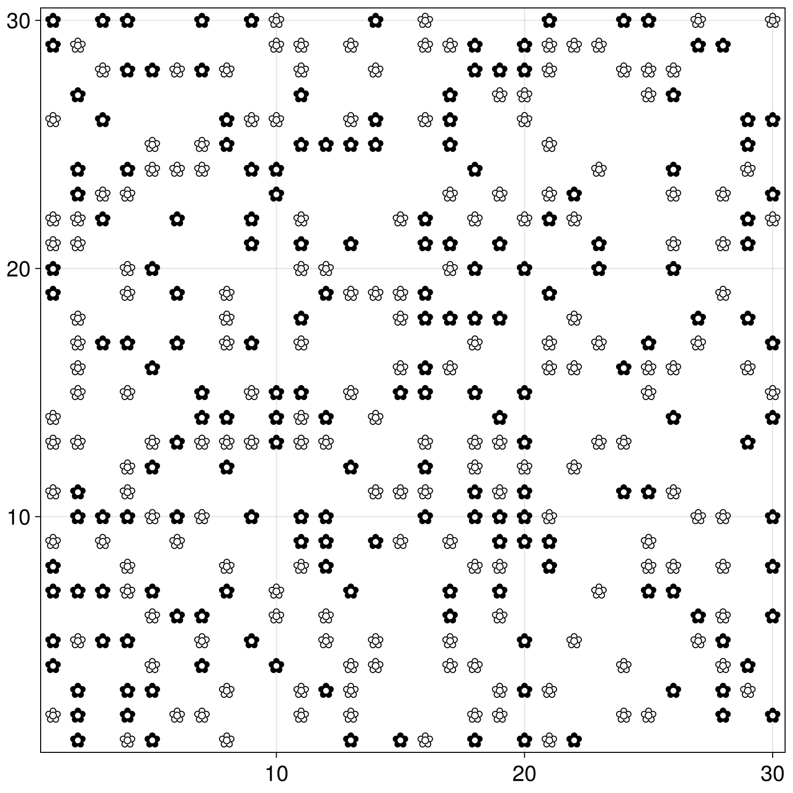
We do not check internally, if the keyword arguments passed to abmplot are supported. Please make sure that there are no typos and that the used kwargs are supported by the abmplot function. Otherwise they will be ignored. This is an unfortunate consequence of how Makie.jl recipes work, and we believe that in the future this problem will be addressed in Makie.jl.
Besides agents, we can also plot spatial properties as a heatmap. Here we plot the temperature of the planet by providing the name of the property as the "heat array":
heatarray = :temperature
heatkwargs = (colorrange = (-20, 60), colormap = :thermal)
plotkwargs = (;
agent_color = daisycolor, agent_size, agent_marker,
agentsplotkwargs = (strokewidth = 1.0,),
heatarray, heatkwargs, colorbar_label = "temperature",
)
fig, ax, abmobs = abmplot(model; plotkwargs...)
fig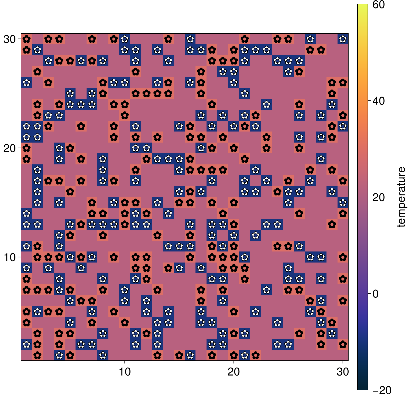
Agents.abmplot — Function
abmplot(model::ABM; kwargs...) → fig, ax, abmobs
abmplot!(ax::Axis/Axis3, model::ABM; kwargs...) → abmobsPlot an agent based model by plotting each individual agent as a marker and using the agent's position field as its location on the plot. abmplot is also used to launch interactive GUIs for evolving agent based models, see "Interactivity" below.
See also abmvideo and abmexploration.
abmplot returns an instance of ABMObservable that can be used to manually animate the model evolution, or make custom composite plots and videos. See the online documentation for examples on using this. Instead of model::ABM, an instance of ABMObservable can also be given to abmplot directly.
Keyword arguments
Agent related
agent_color, agent_size, agent_marker: These three keywords decide the color, size, and marker, that each agent will be plotted as. They can each be either a constant or a function, which takes as an input a single agent and outputs the corresponding value. If the model uses aGraphSpace,agent_color, agent_size, agent_markerfunctions instead take an iterable of agents in each position (i.e. node of the graph).Example using constants:
agent_color = "#338c54", agent_size = 15, agent_marker = :diamondExample using functions:
agent_color(a) = a.status == :S ? "#2b2b33" : a.status == :I ? "#bf2642" : "#338c54" agent_size(a) = 10rand() agent_marker(a) = a.status == :S ? :circle : a.status == :I ? :diamond : :rectFor 2D models,
agent_markercan be/return aMakie.Polygoninstance, which plots each agent as an arbitrary polygon. It is assumed that the origin (0, 0) is the agent's position when creating the polygon. In this case, the keywordagent_sizeis ignored, as each polygon has its own size. Use the functionsscale, rotate_polygonto transform this polygon.3D models currently do not support having different markers. As a result,
agent_markercannot be a function. It should be aMeshor 3D primitive (such asSphereorRect3D).offset = nothing: If notnothing, it must be a function taking as an input an agent and outputting an offset position tuple to be added to the agent's position (which matters only if there is overlap).agentsplotkwargs = NamedTuple(): Additional keyword arguments propagated to the function that plots the agents (typicallyscatter!).
Extra plots related
heatarray = nothing: A keyword that plots a model property (that is a matrix) as a heatmap over the space. Its values can be standard data accessors given to functions likerun!, i.e. either a symbol (directly obtain model property) or a function of the model. If the space isAbstractGridSpacethen matrix must be the same size as the underlying space. ForContinuousSpaceany size works and will be plotted over the space extent. For exampleheatarray = :temperatureis used in the Daisyworld example. But you could also definef(model) = create_matrix_from_model...and setheatarray = f. The heatmap will be updated automatically during model evolution in videos and interactive applications.heatkwargs = NamedTuple(): Keywords given toMakie.heatmapfunction ifheatarrayis not nothing.add_colorbar = true: Whether or not a Colorbar should be added to the right side of the heatmap ifheatarrayis not nothing. It is strongly recommended to useabmplotinstead of theabmplot!method if you useheatarray, so that a colorbar can be placed naturally.colorbar_label = "": Label to add to the colorbar, if any.preplot!: A functionf(ax, abmobs)that plots something after the heatmap, and after space-specific plotting, but before the agents.spaceplotkwargs = NamedTuple(): keywords utilized when plotting the space, if the space extends thespaceplot!function (currently onlyOpenStreetMapSpace).adjust_aspect = true: Adjust axis aspect ratio to be the model's space data aspect ratio.
The stand-alone function abmplot also takes two optional NamedTuples named figure and axis which can be used to change the automatically created Figure and Axis objects.
Interactivity
Evolution related
add_controls::Bool: Iftrue,abmplotswitches to "interactive application GUI" mode where the model evolves interactively usingAgents.step!.add_controlsis by defaultfalseunlessparams(see below) is not empty.add_controlsis also alwaystrueinabmexploration. The application has the following interactive elements:- "step": advances the simulation once for
dttime. - "run": starts/stops the continuous evolution of the model.
- "reset model": resets the model to its initial state from right after starting the interactive application.
- Two sliders control the animation speed: "dt" decides how much time to evolve the model before the plot is updated, and "sleep" the
sleep()time between updates.
- "step": advances the simulation once for
enable_inspection = add_controls: Iftrue, enables agent inspection on mouse hover.dt = 1:50: The values of the "dt" slider which is the time to step the model forwards in each frame update, which callsstep!(model, dt). This defaults to1:50for discrete time models and to0.1:0.1:10.0for continuous time ones.params = Dict(): This is a dictionary which decides which parameters of the model will be configurable from the interactive application. Each entry ofparamsis a pair ofSymbolto anAbstractVector, and provides a range of possible values for the parameter named after the given symbol (see example online). Changing a value in the parameter slides is only propagated to the actual model after a press of the "update" button.
Data collection related
adata, mdata, when: Same as the keyword arguments ofAgents.run!. If either or bothadata, mdataare given, data are collected and stored in theabmobs, seeABMObservable. The same keywords provide the data plots ofabmexploration. This also adds the button "clear data" which deletes previously collected agent and model data by emptying the underlyingDataFramesadf/mdf. Reset model and clear data are independent processes.
See the documentation string of ABMObservable for custom interactive plots.
Interactive ABM Applications
Continuing from the Daisyworld plots above, we can turn them into interactive applications straightforwardly, simply by setting the keyword add_controls = true as discussed in the documentation of abmplot. Note that GLMakie should be used instead of CairoMakie when wanting to use the interactive aspects of the plots!
using GLMakiefig, ax, abmobs = abmplot(model; add_controls = true, plotkwargs...)
fig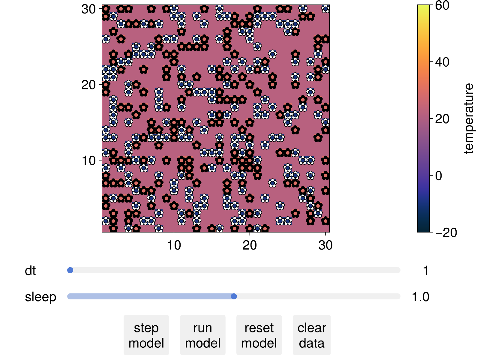
One could click the run button and see the model evolve. Furthermore, one can add more sliders that allow changing the model parameters. This is done by providing a dictionary mapping parameter keys to range of values. When such a dictionary is provided, abmplot goes into interactive mode by default.
params = Dict(
:surface_albedo => 0:0.01:1,
:solar_change => -0.1:0.01:0.1,
)
fig, ax, abmobs = abmplot(model; params, plotkwargs...)
fig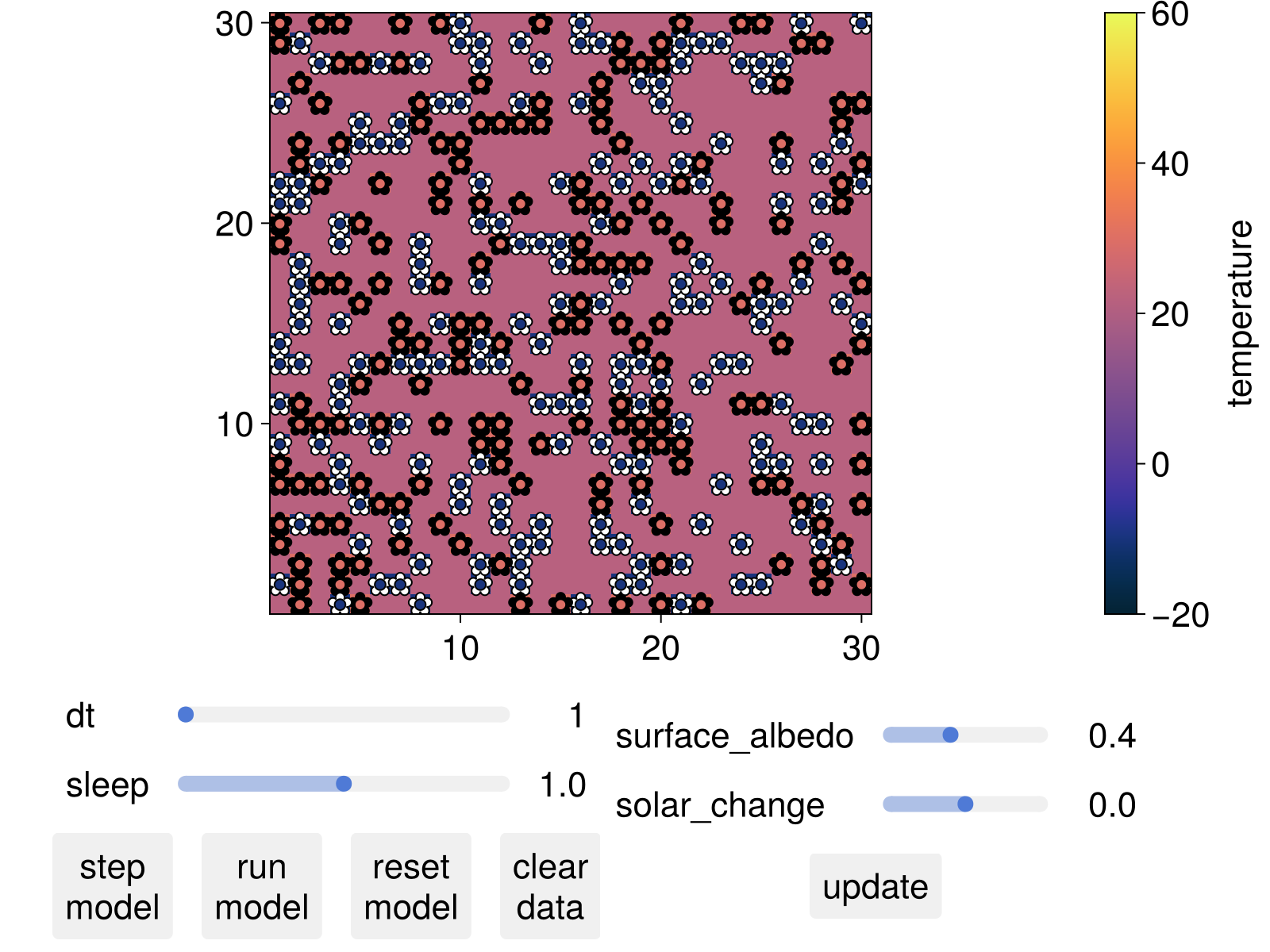
One can furthermore collect data while the model evolves and visualize them using the convenience function abmexploration
using Statistics: mean
black(a) = a.breed == :black
white(a) = a.breed == :white
adata = [(black, count), (white, count)]
temperature(model) = mean(model.temperature)
mdata = [temperature, :solar_luminosity]
fig, abmobs = abmexploration(
model;
params, plotkwargs..., adata, alabels = ["Black daisys", "White daisys"],
mdata, mlabels = ["T", "L"]
)Agents.abmexploration — Function
abmexploration(model::ABM; alabels, mlabels, kwargs...)Open an interactive application for exploring an agent based model and the impact of changing parameters on the time evolution. Requires Agents.
The application evolves an ABM interactively and plots its evolution, while allowing changing any of the model parameters interactively and also showing the evolution of collected data over time (if any are asked for, see below). The agent based model is plotted and animated exactly as in abmplot, and the model argument as well as splatted kwargs are propagated there as-is. This convencience function only works for aggregated agent data.
Calling abmexploration returns: fig::Figure, abmobs::ABMObservable. So you can save and/or further modify the figure and it is also possible to access the collected data (if any) via the ABMObservable.
Clicking the "reset" button will add a red vertical line to the data plots for visual guidance.
Keywords arguments (in addition to those in abmplot)
alabels, mlabels: If data are collected from agents or the model withadata, mdata, the corresponding plots' y-labels are automatically named after the collected data. It is also possible to providealabels, mlabels(vectors of strings with exactly same length asadata, mdata), and these labels will be used instead.figure = NamedTuple(): Keywords to customize the created Figure.axis = NamedTuple(): Keywords to customize the created Axis.plotkwargs = NamedTuple(): Keywords to customize the styling of the resultingscatterlinesplots.
ABM Videos
Agents.abmvideo — Function
abmvideo(file, model; kwargs...)This function exports the animated time evolution of an agent based model into a video saved at given path file, by recording the behavior of the interactive version of abmplot (without sliders). The plotting is identical as in abmplot and applicable keywords are propagated.
Keywords
dt = 1: Time to evolve between each recorded frame. ForStandardABMthis must be an integer and it is identical to how many steps to take per frame.framerate = 30: The frame rate of the exported video.frames = 300: How many frames to record in total, including the starting frame.title = "": The title of the figure.showstep = true: If current step should be shown in title.figure = NamedTuple(): Figure related keywords (e.g. resolution, backgroundcolor).axis = NamedTuple(): Axis related keywords (e.g. aspect).recordkwargs = NamedTuple(): Keyword arguments given toMakie.record. You can use(compression = 1, profile = "high")for a higher quality output, and prefer theCairoMakiebackend. (compression 0 results in videos that are not playable by some software)kwargs...: All other keywords are propagated toabmplot.
E.g., continuing from above,
model = AgentsExampleZoo.daisyworld()
abmvideo("daisyworld.mp4", model; title = "Daisy World", frames = 150, plotkwargs...)You could of course also explicitly use abmplot in a record loop for finer control over additional plot elements.
Creating custom ABM plots
The existing convenience function abmexploration will always display aggregated collected data as scatterpoints connected with lines. In cases where more granular control over the displayed plots is needed, we need to take a few extra steps and utilize the ABMObservable returned by abmplot. The same steps are necessary when we want to create custom plots that compose animations of the model space and other aspects.
Agents.ABMObservable — Type
ABMObservable(model; adata, mdata, when = true) → abmobsabmobs contains all information necessary to step an agent based model interactively, as well as collect data while stepping interactively. ABMObservable also returned by abmplot.
Calling Agents.step!(abmobs, t) will step the model for t time and collect data as in Agents.run!, using the adata, mdata, when keywords. The fields abmobs.model, abmobs.adf, abmobs.mdf are observables that contain the AgentBasedModel, and the agent and model dataframes with collected data. These observables are updated (and notify) during step!.
All plotting and interactivity should be defined by lift-ing (or map-ing) these observables according to the Observables.jl interface.
To do custom animations you need to have a good idea of how Makie's animation system works. Have a look at this tutorial if you are not familiar yet.
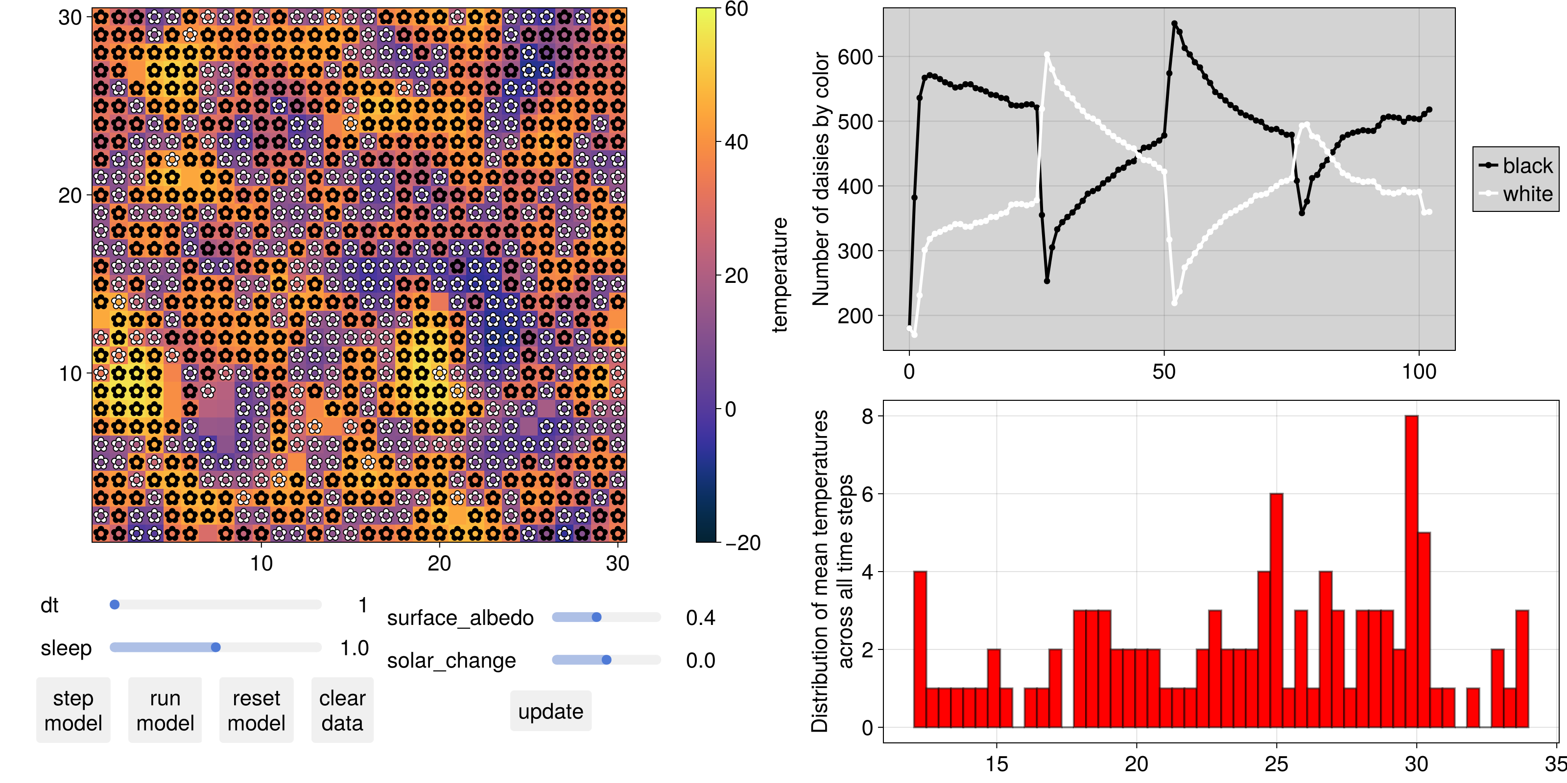
create a basic abmplot with controls and sliders
model = AgentsExampleZoo.daisyworld(; solar_luminosity = 1.0, solar_change = 0.0, scenario = :change)
fig, ax, abmobs = abmplot(
model; params, plotkwargs...,
adata, mdata, figure = (; size = (1600, 800))
)
fig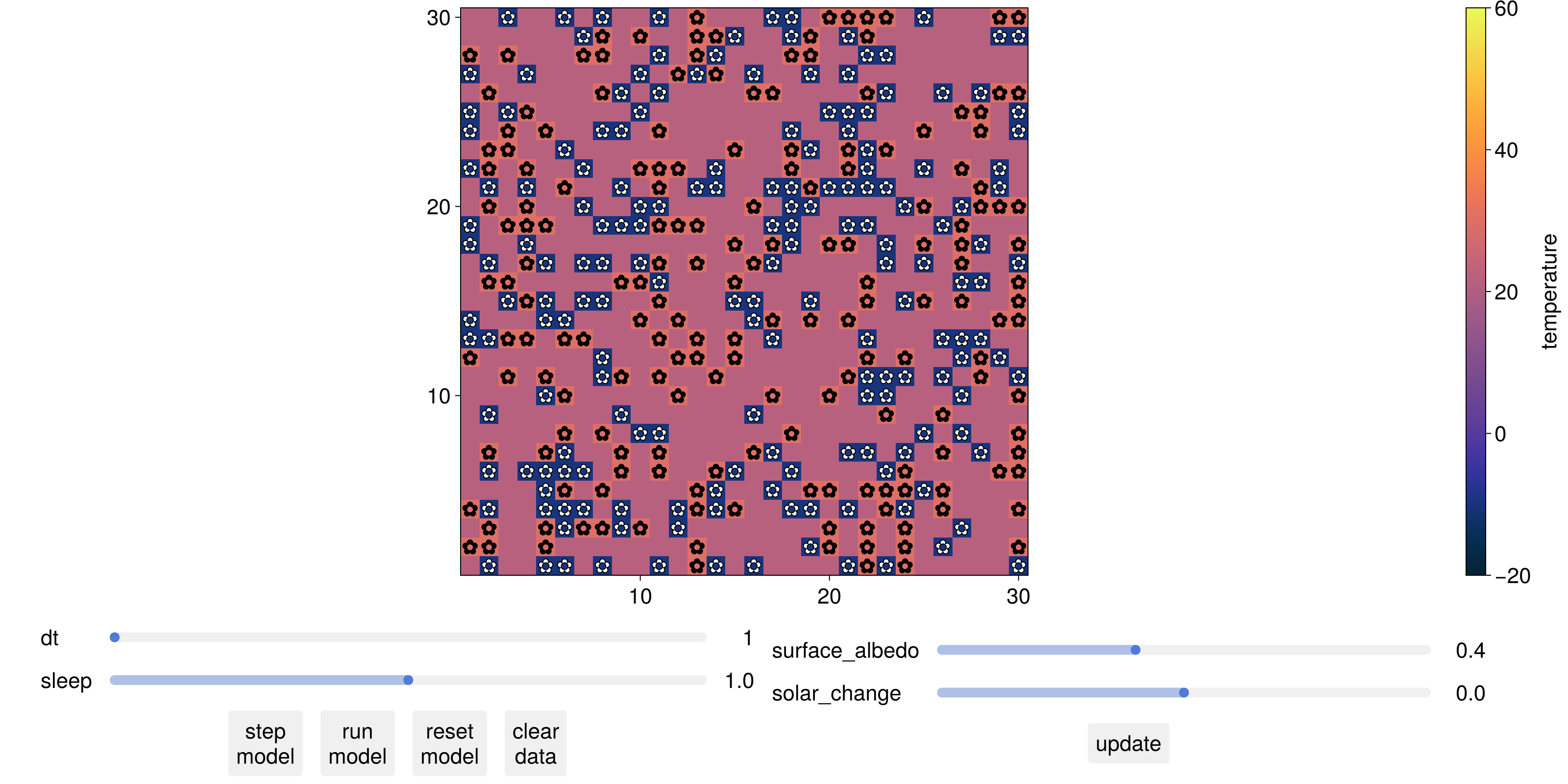
abmobsABMObservable with model:
StandardABM with 360 agents of type Daisy
 agents container: Dict
 space: GridSpaceSingle with size (30, 30), metric=chebyshev, periodic=true
 scheduler: fastest
 properties: temperature, solar_luminosity, max_age, surface_albedo, ratio, solar_change, tick, scenario
and with data collection:
adata: Tuple{Function, typeof(count)}[(Main.black, count), (Main.white, count)]
mdata: Any[Main.temperature, :solar_luminosity]create a new layout to add new plots to the right of the abmplot
plot_layout = fig[:, end + 1] = GridLayout()GridLayout[1:1, 1:1] with 0 children
create a sublayout on its first row and column
count_layout = plot_layout[1, 1] = GridLayout()GridLayout[1:1, 1:1] with 0 children
collect tuples with x and y values for black and white daisys
blacks = @lift(Point2f.($(abmobs.adf).time, $(abmobs.adf).count_black))
whites = @lift(Point2f.($(abmobs.adf).time, $(abmobs.adf).count_white))
Observable(Point{2, Float32}[[0.0, 180.0]])
create an axis to plot into and style it to our liking
ax_counts = Axis(
    count_layout[1, 1];
    backgroundcolor = :lightgrey, ylabel = "Number of daisies by color"
)
Axis with 0 plots:
plot the data as scatterlines and color them accordingly
scatterlines!(ax_counts, blacks; color = :black, label = "black")
scatterlines!(ax_counts, whites; color = :white, label = "white")
Plot{Makie.scatterlines, Tuple{Vector{Point{2, Float32}}}}add a legend to the right side of the plot
Legend(count_layout[1, 2], ax_counts; bgcolor = :lightgrey)Legend()and another plot, written in a more condensed format
ax_hist = Axis(
    plot_layout[2, 1];
    ylabel = "Distribution of mean temperatures\nacross all time steps"
)
hist!(
    ax_hist, @lift($(abmobs.mdf).temperature);
    bins = 50, color = :red,
    strokewidth = 2, strokecolor = (:black, 0.5),
)

fig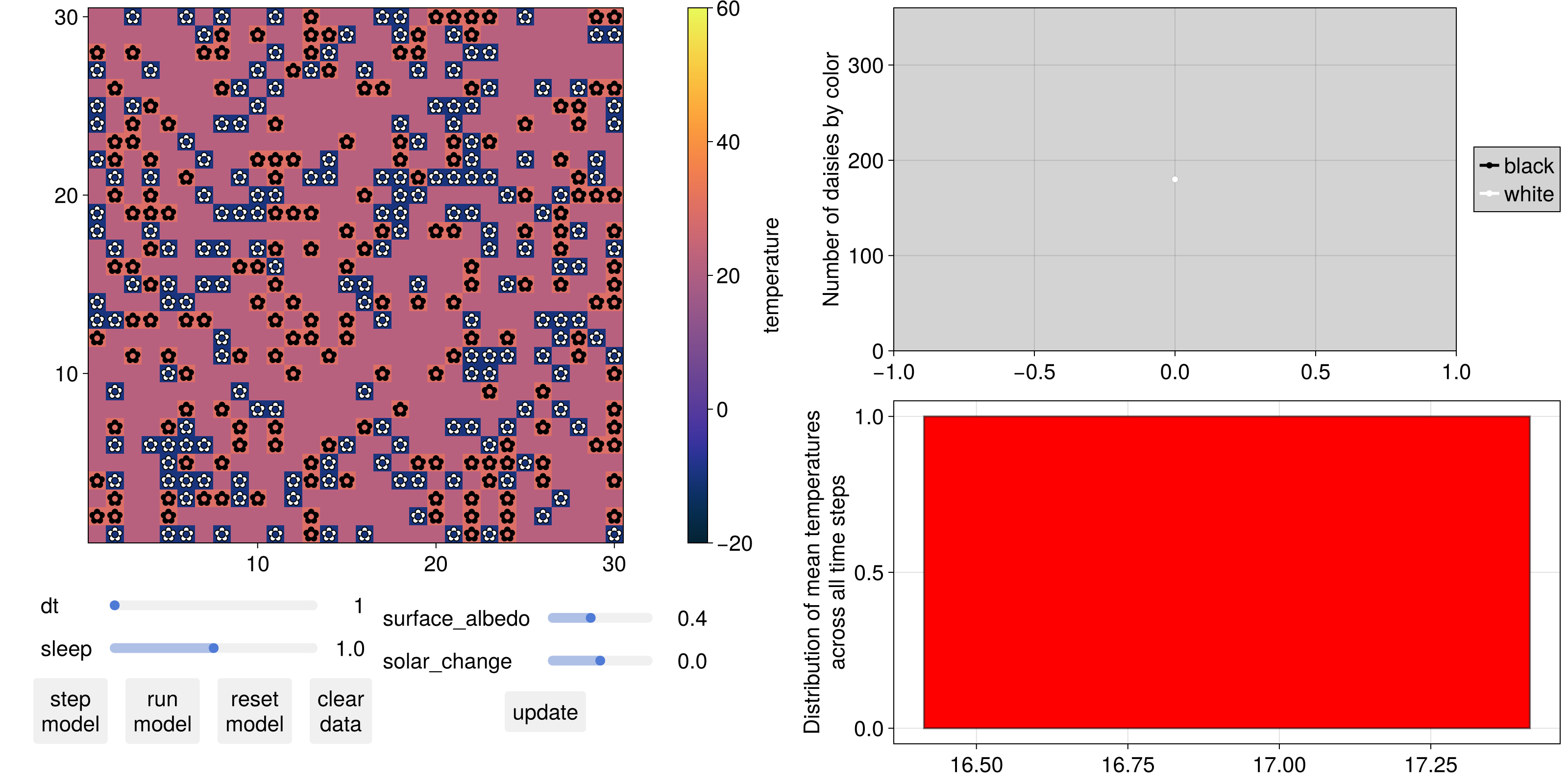
Now, once we step the abmobs::ABMObservable, the whole plot will be updated
Agents.step!(abmobs, 1)
Agents.step!(abmobs, 1)
fig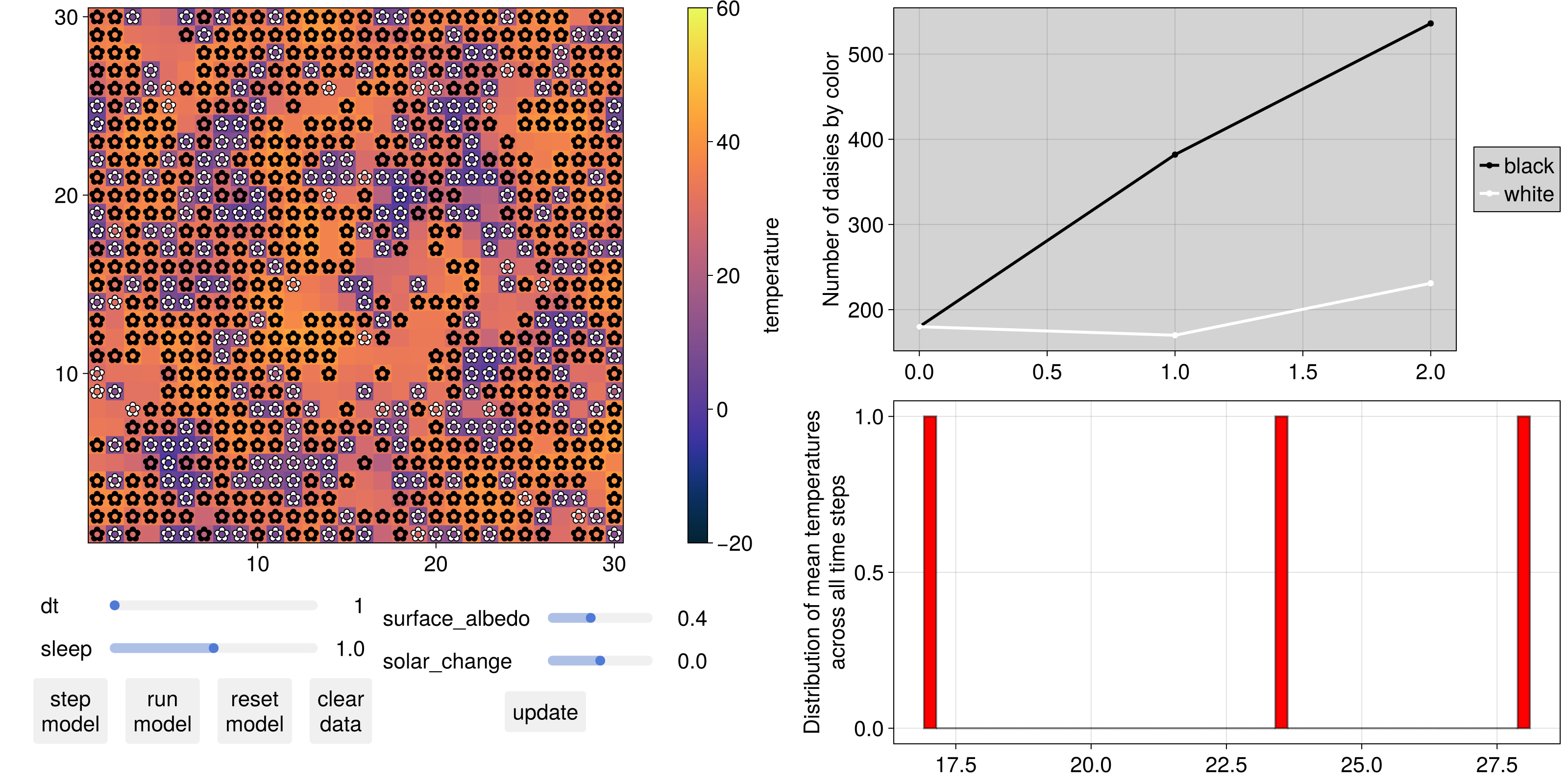
Of course, you need to actually adjust axis limits given that the plot is interactive
autolimits!(ax_counts)
autolimits!(ax_hist)
Or, simply trigger them on any update to the model observable:
on(abmobs.model) do m
    autolimits!(ax_counts)
    autolimits!(ax_hist)
end
ObserverFunction defined at agents_visualizations.md:281 operating on Observable(StandardABM with 767 agents of type Daisy
agents container: Dict
space: GridSpaceSingle with size (30, 30), metric=chebyshev, periodic=true
scheduler: fastest
properties: temperature, solar_luminosity, max_age, surface_albedo, ratio, solar_change, tick, scenario)and then marvel at everything being auto-updated by calling step! :)
for i in 1:100
    step!(abmobs, 1)
end
fig